What "Thinking" Really Is: Lessons from an AI That Solves Sliding Puzzles
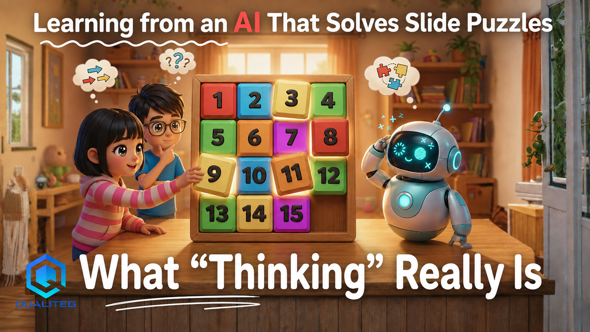
Hello!
"Apparently this puzzle appears in AI textbooks."
The sliding puzzle you played with as a kid. Actually, it is plenty of fun for adults too.
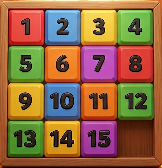
You know the one—you click numbered tiles around until they line up. Did you know this simple puzzle was one of the starting points of AI research?
In this article, we use this puzzle to unravel how an AI "thinks." What's more, the techniques involved underpin all sorts of modern technology, from route finding in Google Maps to ChatGPT.
First, Let's Play
Before the theory, let's refresh your intuition.
Click shuffle to scramble the board and start the game.
Every shuffle is guaranteed to be solvable, by the way—though if you are out of practice it can be fairly challenging.
How did it go?
How many moves did it take you?
Don't worry if you couldn't solve it. In the second half of the article, there is a version of the game where the AI solves it for you.
Here is a video. You can watch the algorithm introduced in this post actually solving the puzzle.
In the second half of the article, we actually implement the algorithm, like this
While you were solving it, what were you thinking? Probably something like "just going by feel," "working from the edges," or "I remember the patterns."
As it turns out, mathematically unraveling what that "going by feel" really is was one of the starting points of AI research.
How Humans Solve It
When a human solves the puzzle, it goes roughly like this.
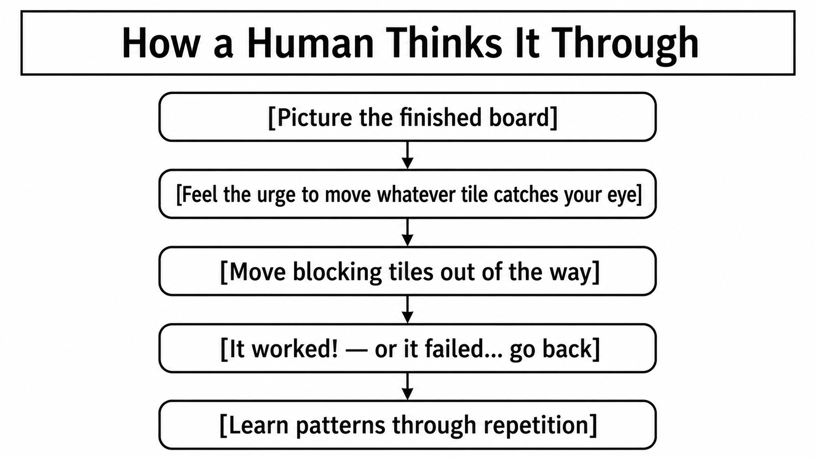
This is a very "local" approach. You are not computing the globally shortest path; you are solving the problem right in front of you, one step at a time. The human brain is good at this kind of intuitive processing, and it works reasonably well.
So how does a computer approach it?
The AI View: Seeing the World as "States"
A computer sees the 15-puzzle like this.
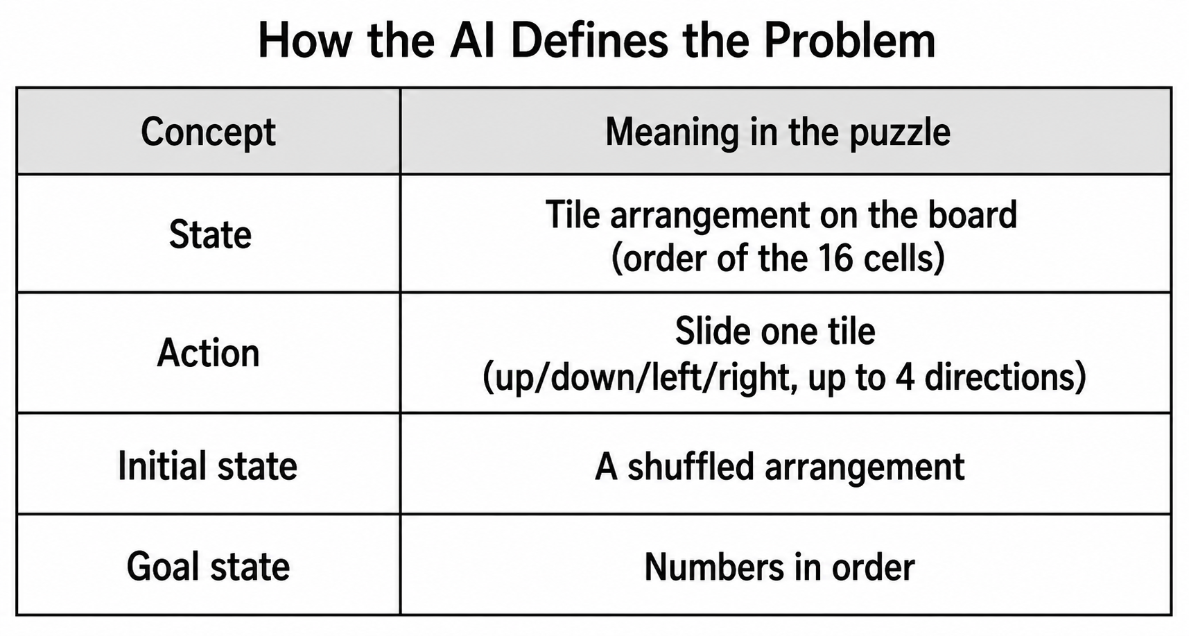
Why Think in "States"?
The key here is the idea of reframing the problem as "transitions between states".
A human thinks "move the tiles", but
a computer thinks "move from one arrangement to another."
Why does this change of perspective matter? Because it lets us handle the problem within the framework of graph theory.
Graph theory is the branch of mathematics that studies the relationships between points (nodes) and lines (edges). If we treat each puzzle arrangement as a point and each single-move relationship as a line, then solving the puzzle becomes "finding a route from the start point to the goal point"—a mathematically well-studied problem.
That means the path-finding algorithms accumulated over decades of research become directly applicable. This is the strength of the "state-space search" approach.
The Structure of the State Space
Drawn as a diagram, the states branch out into a tree-like structure.
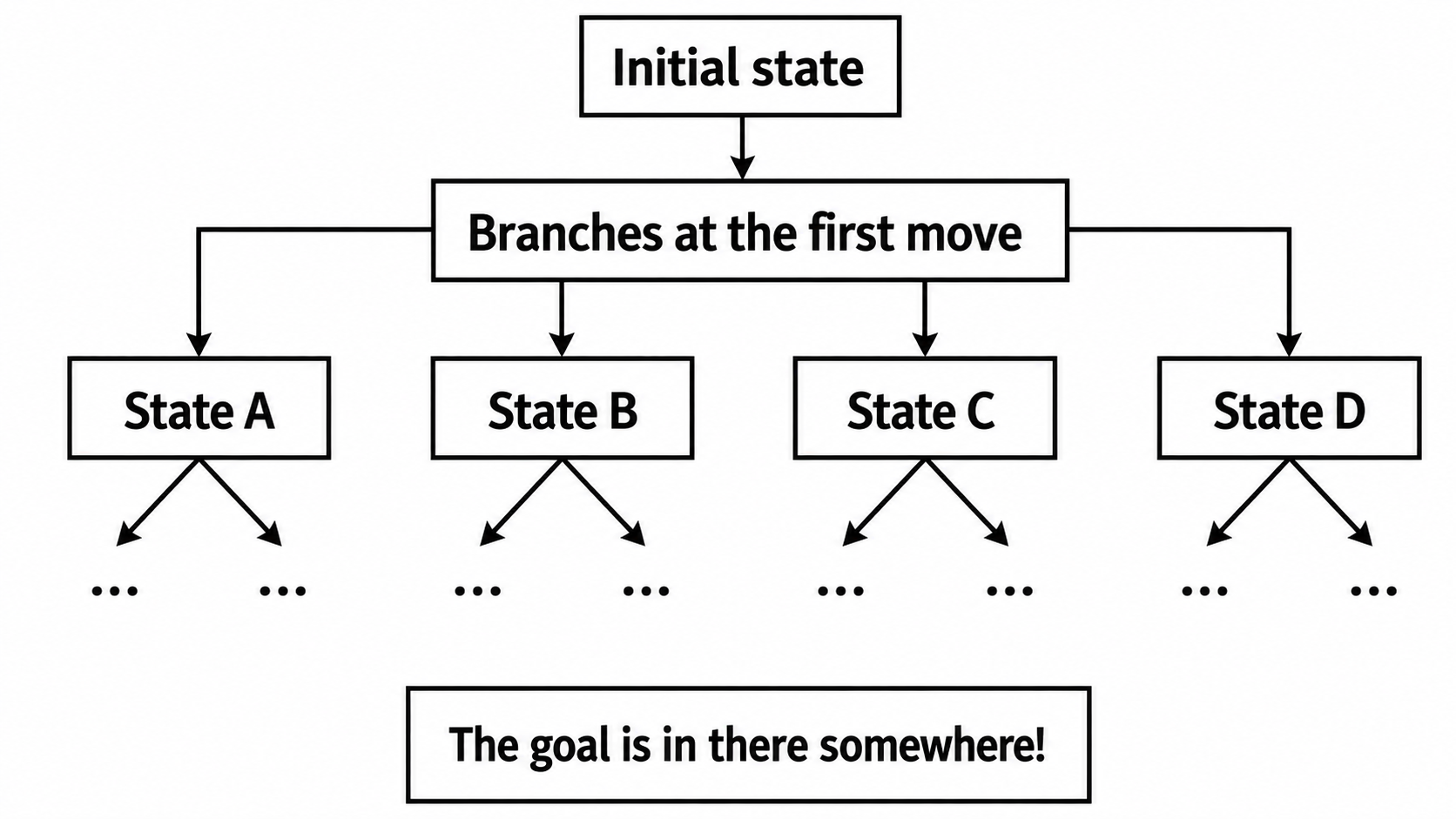
Each move branches into roughly 2 to 4 states. Two moves give up to 16, three moves up to 64... and the possibilities expand exponentially.
Somewhere in this "tree of states" lies the goal. The computer's job is to find the route to it.
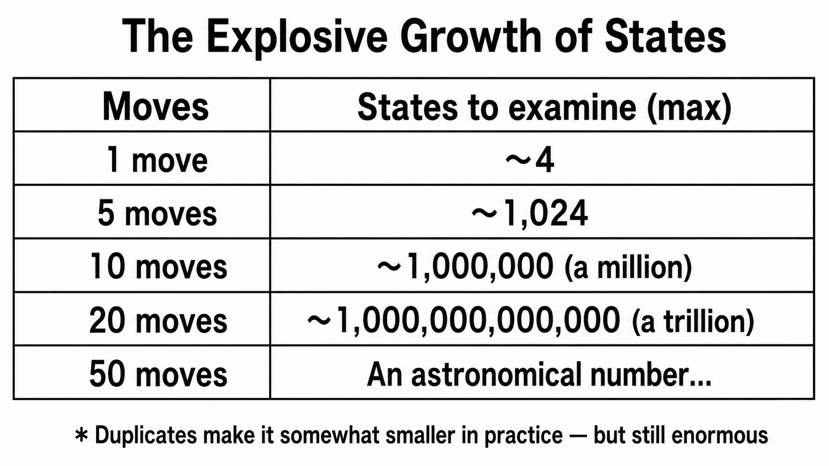
We just used the phrase "grows exponentially." It means that with each additional move, the number of states to examine multiplies. If it quadruples with every move, ten moves give about a million states and twenty moves about a trillion. This explosive growth is the essence of what makes the puzzle hard to solve.
Some Arrangements Cannot Be Solved!?
Here is a fun fact.
The 15-puzzle has arrangements that can never be solved, no matter how hard you try.
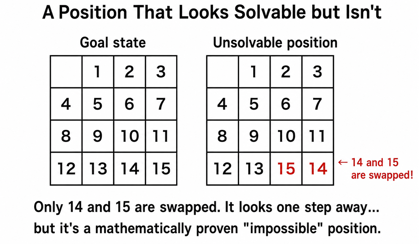
The puzzle was a huge craze in 1880s America. A
"solve it and win a prize!"
contest was even held—but nobody could solve it. The matter was later settled when mathematicians proved that no solution existed in the first place.
Why It Cannot Be Solved: The Inversion Count
The test uses a concept called the "inversion count."
The inversion count is the number of pairs where, scanning the tiles in order, a number that should come later appears earlier.
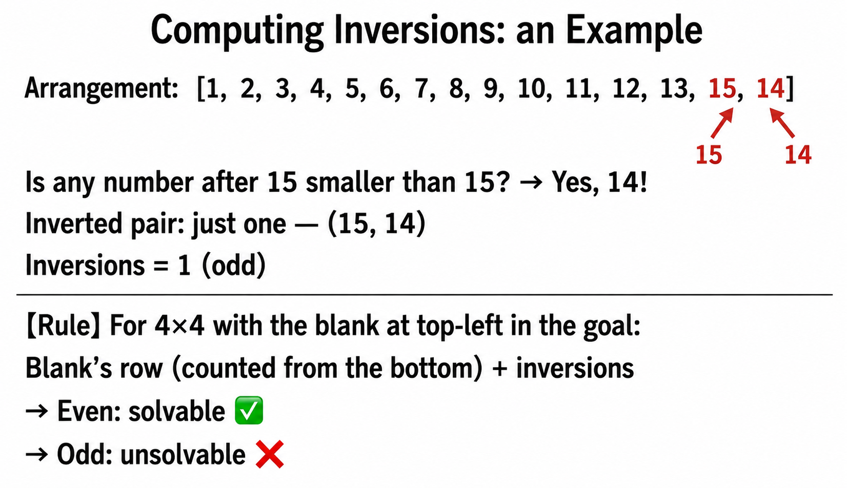
Why Does the Inversion Count Decide It?
This gets a bit mathematical, but let's try an intuitive explanation.
Each time you slide a tile, the inversion count always changes by an odd amount (up by 1, down by 1, or by ±3, and so on). In other words, the parity of the inversion count (even or odd) flips with every single move.
The goal state has an inversion count of 0 (even). That means it can only be reached in an even number of moves. If the initial state has an odd inversion count, no number of moves will ever make it even—so the goal can never be reached.
This is the idea of an "invariant": by finding a property that is preserved no matter how the system changes, you can determine reachability.
The game we built also runs this check behind the scenes and only generates arrangements that are guaranteed solvable. The program makes sure it never hands you an unsolvable problem.
Brute Force vs. Searching Smart
Now that we know an arrangement is solvable, how do we find the solution?
Breadth-First Search (BFS): Try Everything
The simplest method is "breadth-first search."
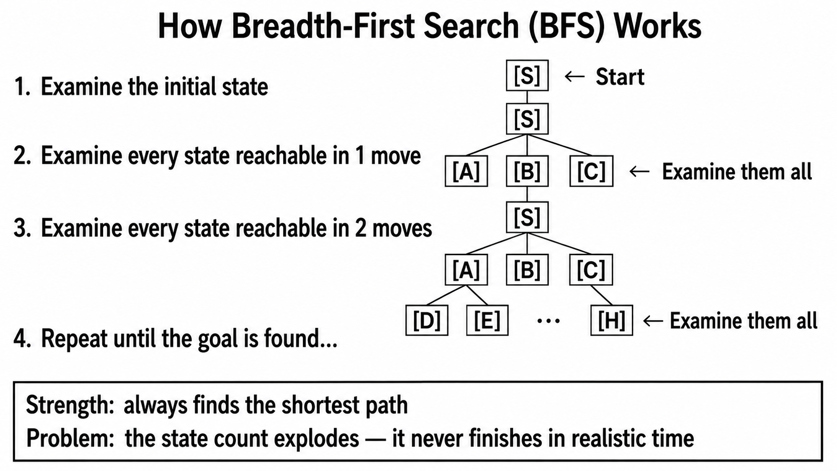
The BFS Algorithm
Let's look at how BFS moves in a bit more detail.
BFS's strategy is "check everything, nearest first." First examine everything reachable in one move, then everything reachable in two moves... proceeding in order of distance (move count).
The greatest advantage of this method is that the shortest path is guaranteed. A state reachable in five moves is always found only after every state within four moves has been examined. So the moment the goal is first found, it is certain to be via a shortest path.
But that "check everything" is the catch. For the 15-puzzle, searching 20 moves deep means examining roughly a trillion states. Even a computer checking a million states per second would need about 12 days.
Not exactly practical.
A* Search (A-star): Using Smart Intuition
Enter "A* (A-star) search." Invented in 1968 by Peter Hart, Nils Nilsson, and Bertram Raphael at Stanford, this algorithm narrows the search using "smart intuition."
The Core Idea of A*
BFS explored in order of fewest moves. A* changes this to "whichever looks likely to reach the goal soonest."
To judge what "looks likely to reach the goal soonest," A* combines two pieces of information.
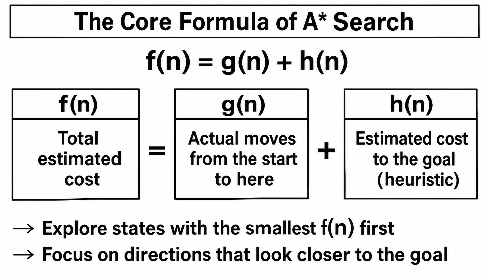
- g(n): how many moves it actually took to get here from the start (a known value)
- h(n): roughly how many more moves it will likely take to reach the goal from here (an estimate)
- f(n): the total—roughly how many moves this route will take to reach the goal
A* explores states with the smallest f(n) first. In other words, it prioritizes the direction that looks cheapest overall.
Why Is This Smart?
If BFS is a "wave spreading in a circle," A* is more like an "ellipse stretching toward the goal."
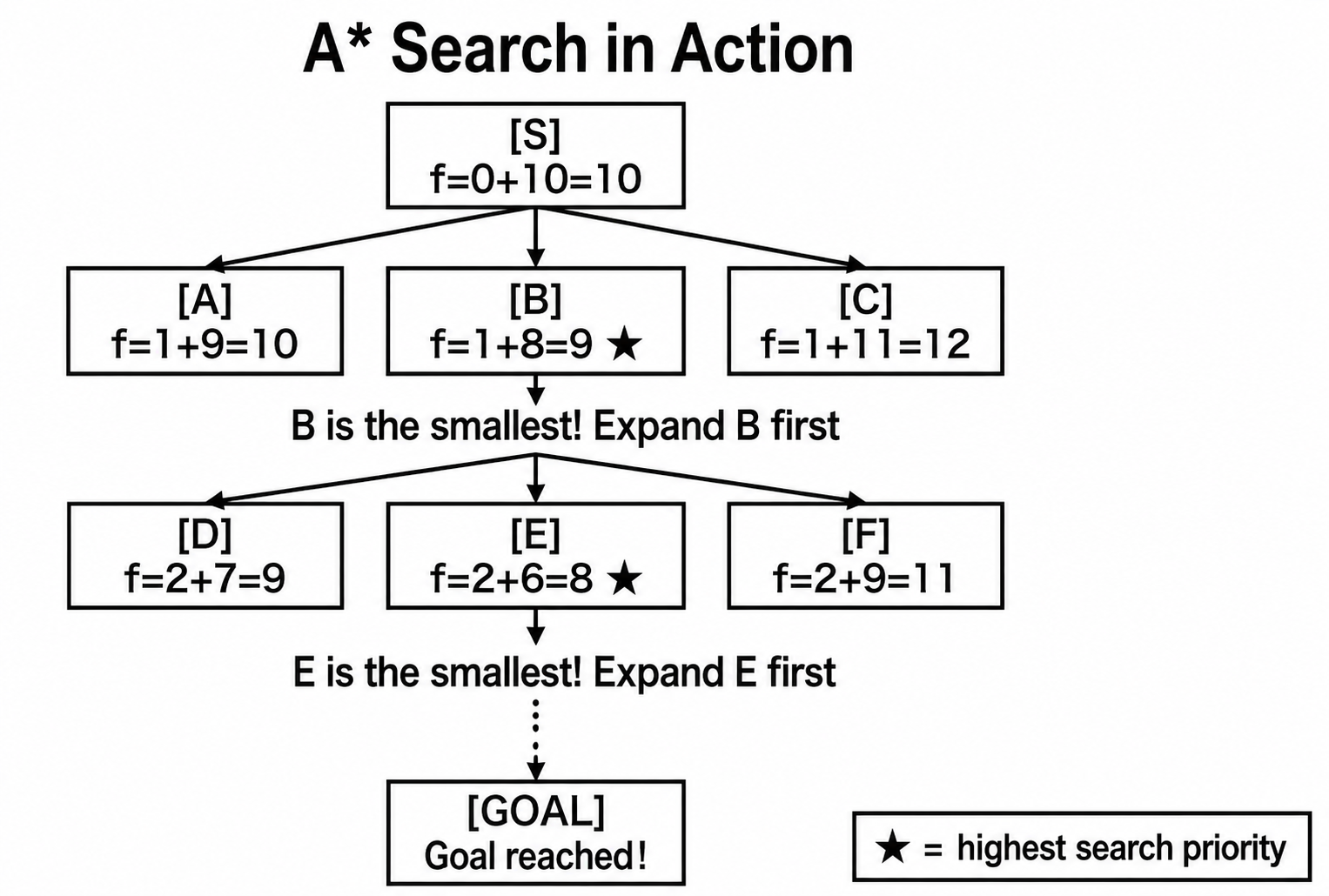
In this example, state B has the smallest f(n) at 9, so B is expanded first. A and C wait their turn. If the goal lies beyond B, we never have to examine A or C at all.
This is the essence of A*'s "smartness."By examining the directions that look closest to the goal first, it can cut out a huge amount of wasted search.
The Heuristic Function: Turning "Intuition" into Numbers
A*'s performance hinges on how h(n) is computed. The function that computes h(n) is called a "heuristic function."
"Heuristic" means "discovery-oriented" or "based on rules of thumb."
It is a "smart guess" that does not guarantee the optimal answer but works well in most cases.
What Makes a Good Heuristic
A heuristic function must satisfy some important conditions.
- It must be fast to compute: it gets evaluated millions of times, so a slow computation ruins everything
- It must return smaller values closer to the goal: otherwise the priorities come out wrong
- It must be admissible: it must never overestimate the actual cost
The third property, "admissible," is especially important. We will explain it in detail shortly.
Manhattan Distance: The 15-Puzzle's "Intuition"
The heuristic most commonly used for the 15-puzzle is "Manhattan distance."
What Is Manhattan Distance?
Manhattan distance is the distance you walk along a grid of streets.
The streets of Manhattan in New York form a grid, so you cannot walk diagonally. The distance when you can only move vertically or horizontally is the Manhattan distance.
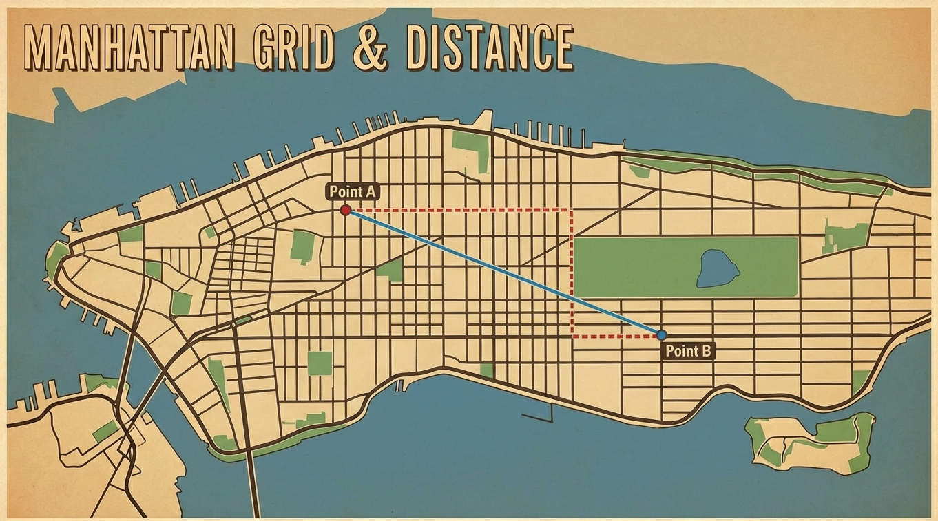
Let's compare it with ordinary straight-line distance (Euclidean distance).
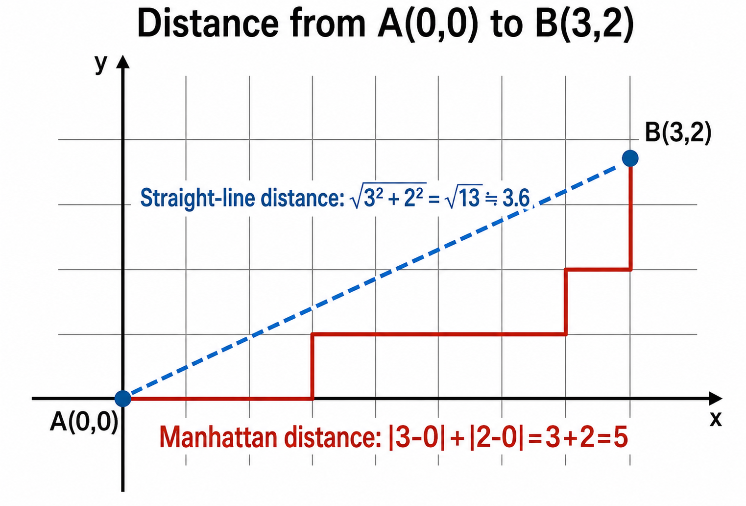
In the 15-puzzle, tiles can only move up, down, left, or right—so Manhattan distance is a perfect fit.
How It Is Computed for the 15-Puzzle
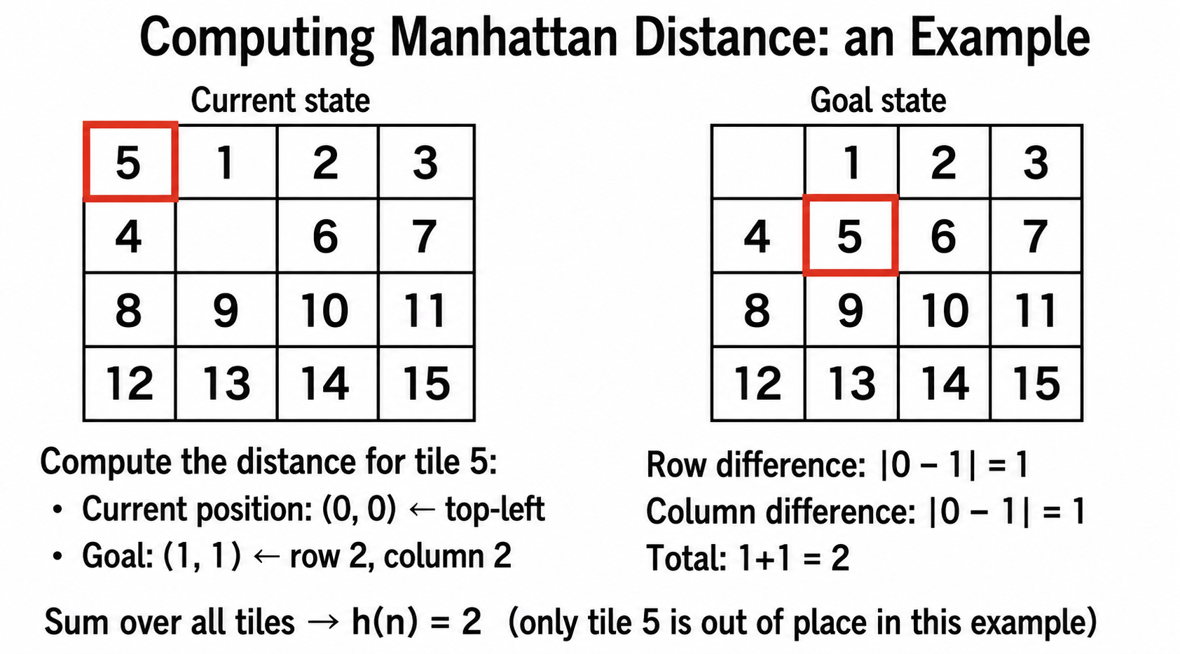
For each tile, compute the Manhattan distance between where it is now and where it should be, and add them all up.
Why Is Manhattan Distance So Good?
There are three reasons Manhattan distance suits the 15-puzzle.
- It is fast to compute: just subtract and add tile coordinates—done in an instant
- It is intuitively correct: if tile 5 is two squares away, you need at least two moves to put it in place. That much is obvious
- It is admissible: this is the crucial one. Manhattan distance gives a lower bound—"you need at least this many moves." In practice, other tiles get in the way and more moves are usually needed, but it absolutely never overestimates
Why Being Admissible Matters
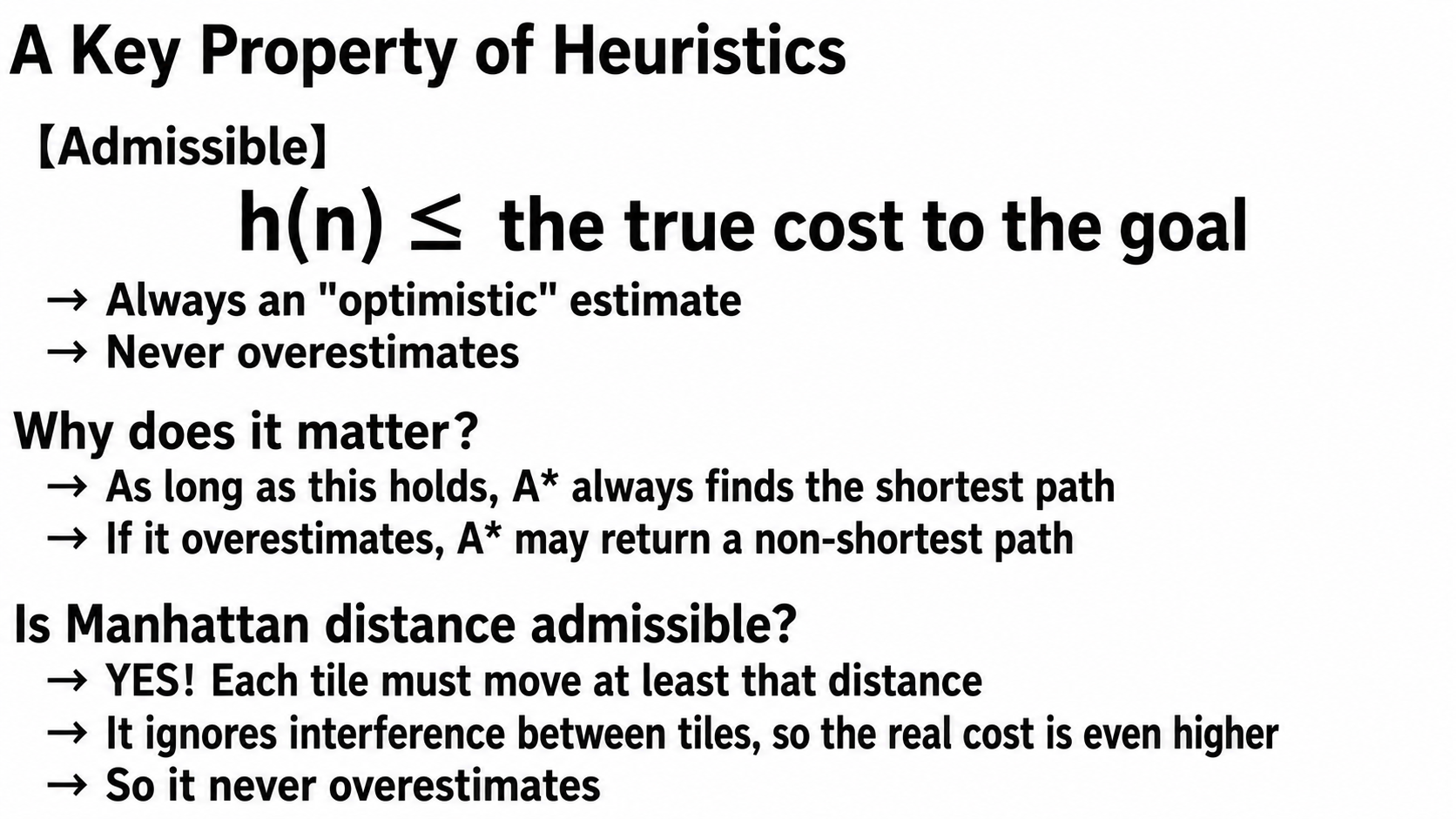
A heuristic function being "admissible" means it never overestimates the actual cost.
Why Must It Never Overestimate?
If h(n) returns a value larger than the actual cost, the algorithm may mistakenly think "this route looks expensive" and postpone what is actually the shortest path. As a result, it can wrongly return a non-shortest route as "the shortest."
Underestimating, on the other hand, is harmless. Even if a route gets examined first because it "looks short," the correct route will still be found later if it turns out to be long.
In other words, a heuristic function should be optimistic. The correct usage is to provide a lower bound: "it will take at least this much."
Manhattan Distance Is Admissible
Manhattan distance provides exactly that lower bound. For tile 5 to travel from position (0,0) to position (1,1), at least two moves are required. Other tiles may force a detour that adds moves, but moving in fewer than two is physically impossible.
That is why Manhattan distance is always "at or below the actual cost"—it is admissible.
A Dramatic Difference in Computation
Let's see just how big the difference is in practice.
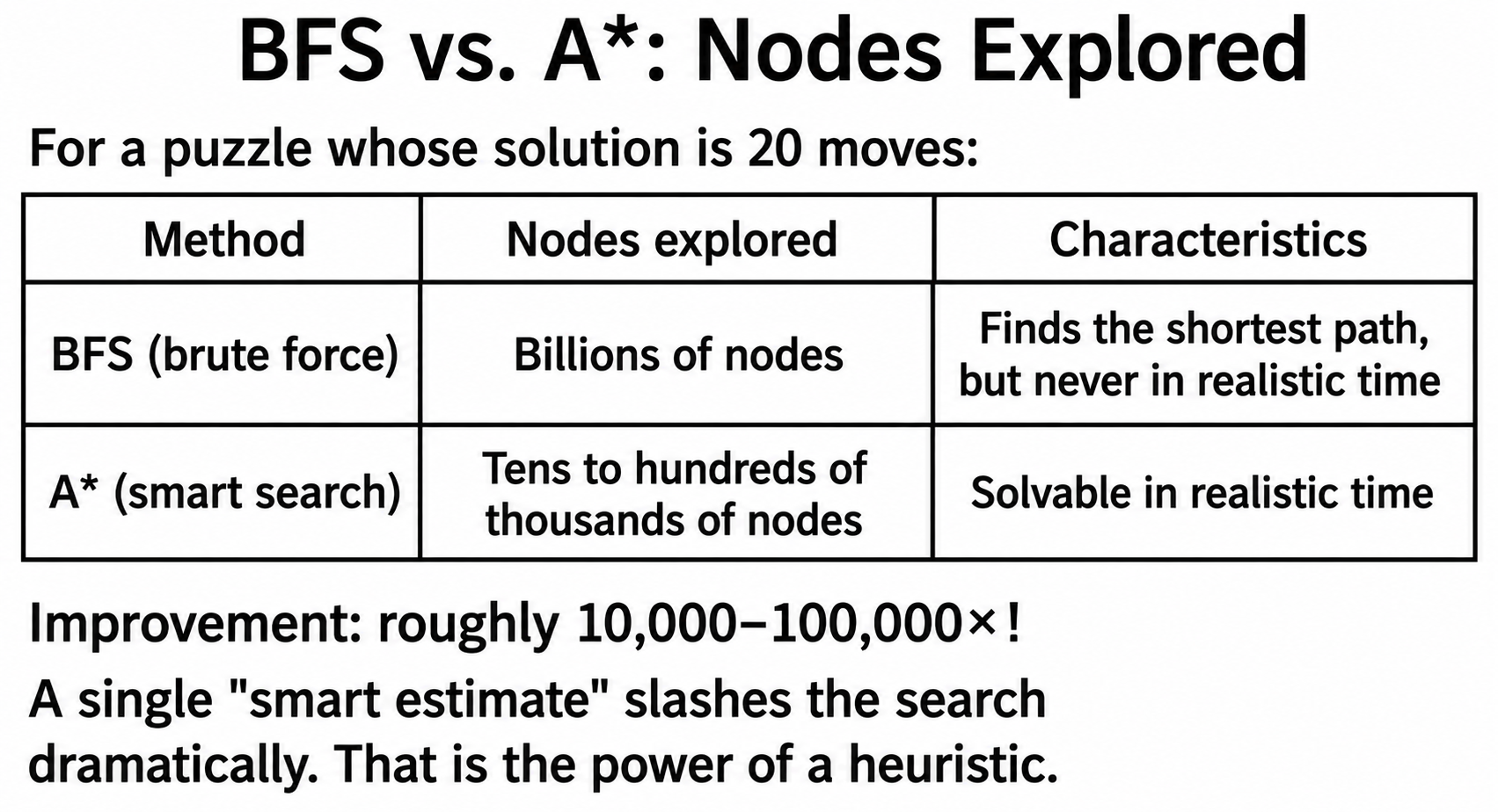
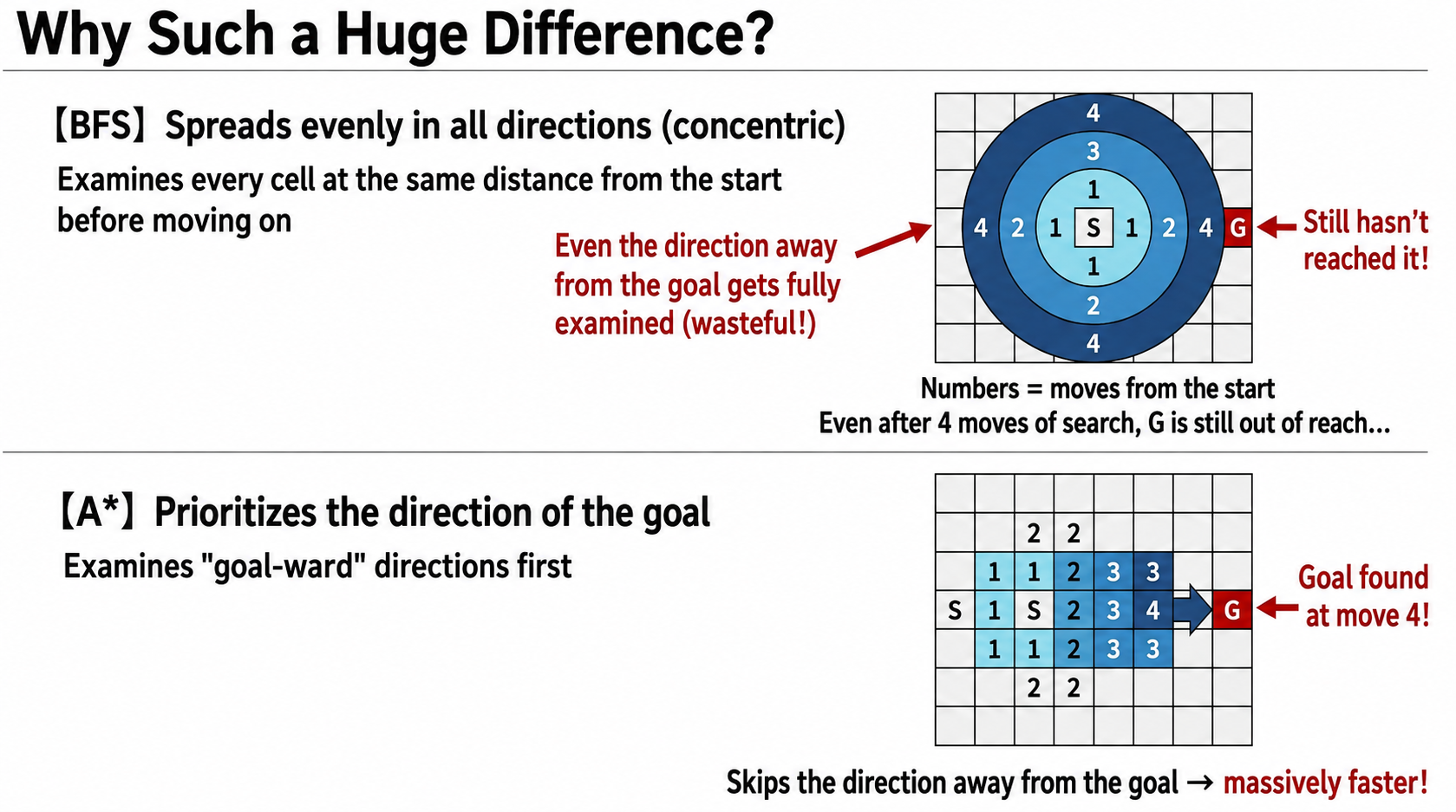
As the figure shows, BFS searches like a circle spreading evenly in all directions, while A* searches like an ellipse stretching toward the goal. Cutting out the wasted search in the directions away from the goal is what produces this enormous difference.
Where Is This Technique Used?
Now for the main event. The techniques we used on the 15-puzzle—state-space search and heuristics—form the foundation of many modern AI technologies.
"AI" is an umbrella term covering deep learning, machine learning, rule-based systems, and more. Where do the techniques from our puzzle fit in?
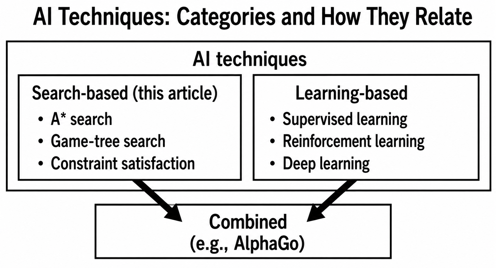
Search-Based vs. Learning-Based
AI techniques divide broadly into "search-based" and "learning-based."
Search-based approaches are used when the problem's structure can be clearly defined. States, actions, and goals are explicit, and the problem is solved by "finding a path to the answer." Our 15-puzzle, chess, and route finding all fall into this category.
Learning-based approaches learn "patterns" from large amounts of data. They suit problems where writing explicit rules is hard—image recognition, speech recognition, recommender systems. Deep learning and random forests belong here.
And today's state-of-the-art AI (AlphaGo, for example) combines the two, acquiring the "smart estimates" used in search through learning.
Concrete Applications
Let's look at each in detail.
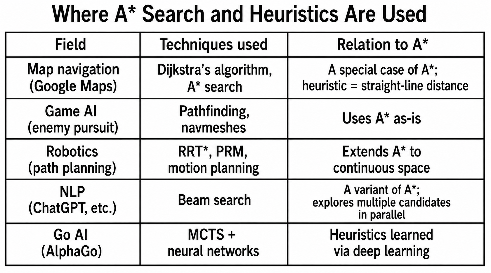
1. Route Finding in Google Maps
The reason your car navigation system or map app produces a route in an instant is A* search.
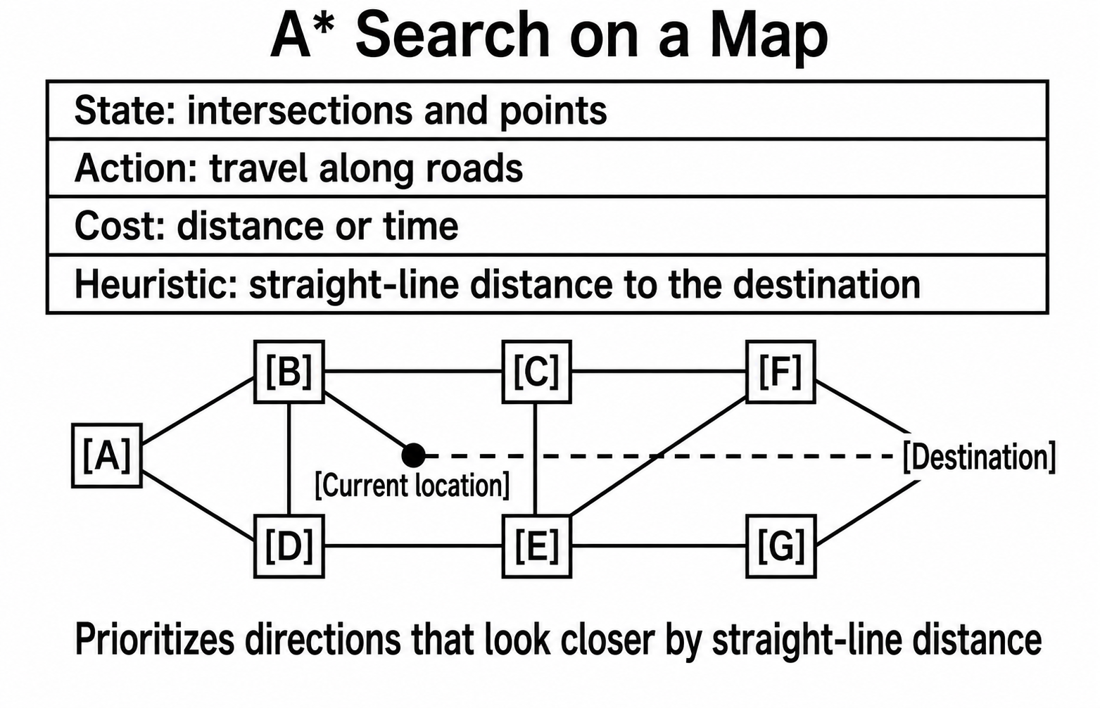
For maps, the heuristic function is "straight-line distance to the destination." Roads twist and turn, but they can never be shorter than the straight line—so the heuristic is admissible.
The real Google Maps applies far more sophisticated optimizations (hierarchical search, precomputation, and so on), but the basic idea is the same as A*.
2. Game AI (Pathfinding)
In RPGs and action games, enemy characters chase the player—closing in along the shortest path while avoiding obstacles. That is A* search too.
In game development this is called "pathfinding," and it comes built into Unity and Unreal Engine.
3. Robot Motion Planning
A robot arm picks up an object and places it somewhere else. Planning that motion also uses state-space search.
For a robot, a "state" is a combination of joint angles. With a 6-axis robot arm, specifying six angles determines the position of the end effector. An "action" is nudging each joint slightly. The "goal" is bringing the end effector to the target position.
A robot's state space is continuous (angles are real numbers), so it differs somewhat from a discrete problem like the 15-puzzle. Algorithms designed for continuous spaces are used instead—RRT* (Rapidly-exploring Random Tree*) and PRM (Probabilistic Roadmap)—but the basic idea of "prioritize directions that look closer to the goal" is the same.
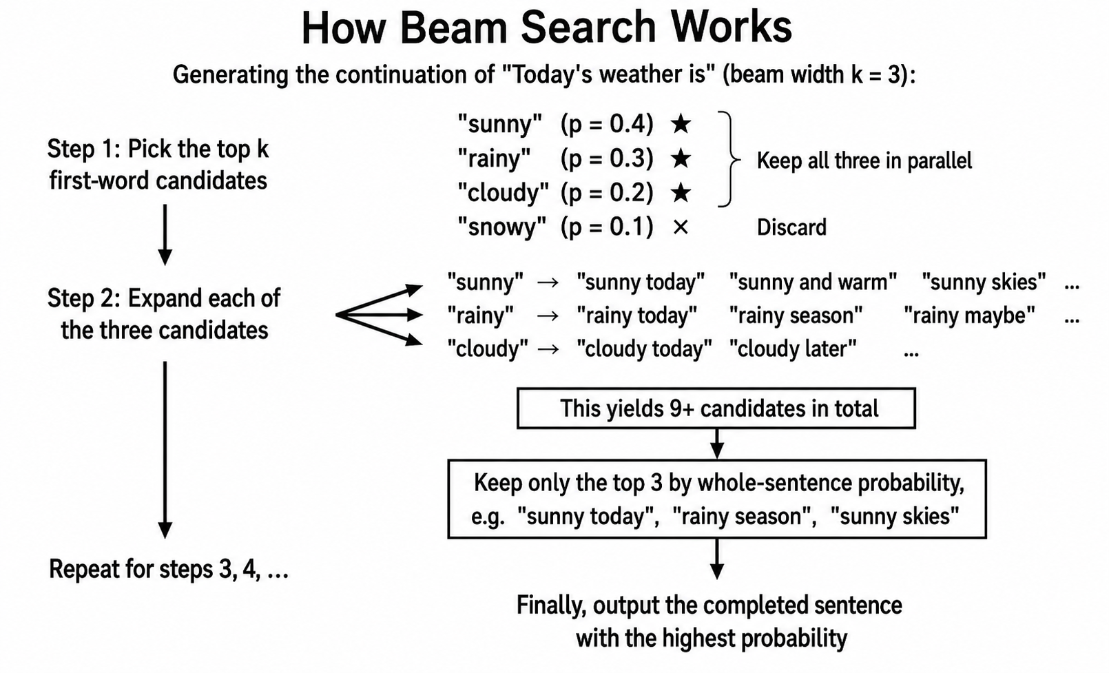
4. Language Models like ChatGPT (Beam Search)
Here is where it gets interesting. When a large language model (LLM) like ChatGPT generates text, a technique called beam search is sometimes used in the process of deciding which word to pick next.
How It Differs from top-k Sampling
There is a similar-sounding term, "top-k," that is well known in LLM circles, so let's sort out the difference.
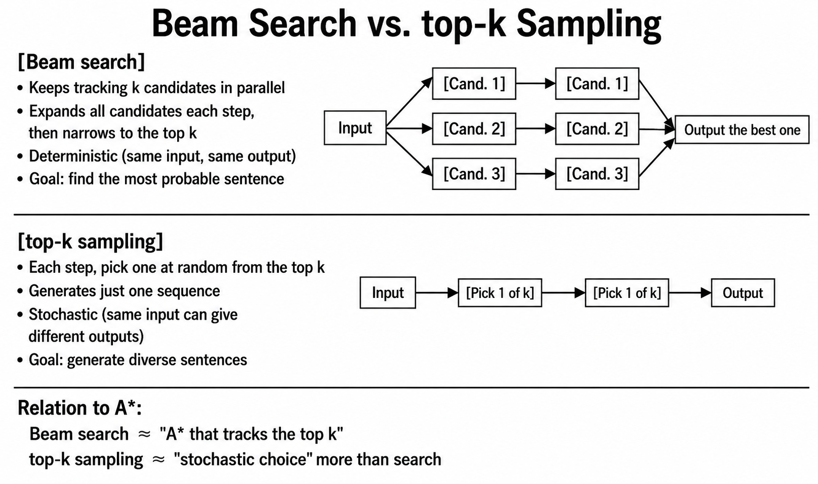
Beam search resembles A in that it prioritizes exploring the most promising candidates. A tracks the single best candidate, while beam search tracks k candidates in parallel—giving it the flexibility to recover mid-way even if the first choice was poor.
[Reference] We also touch on Top-K in the following article explaining LLM sampling
 Qualiteg プロダクト開発部
5. AlphaGo: Search Meets Deep Learning
The Go AI "AlphaGo" was groundbreaking as a fusion of search-based and learning-based approaches.
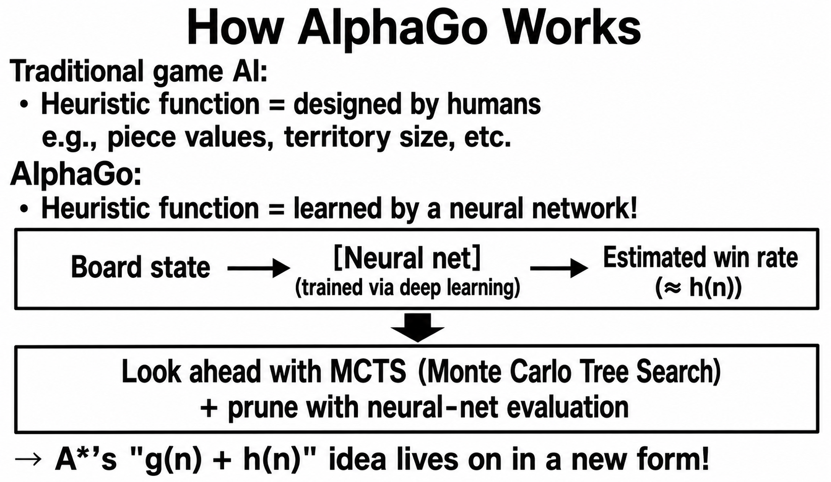
For the 15-puzzle, we used Manhattan distance—a heuristic designed by humans. But for a game as complex as Go, designing a good heuristic function by hand is extremely difficult.
AlphaGo's innovation was to learn this heuristic function automatically with a neural network. From vast game records and self-play, it acquired the ability to judge which side a given board position favors.
In other words, AlphaGo kept the "search" framework intact and replaced the "smart estimation" part with deep learning.
How Do Deep Learning and Random Forests Relate?
"Deep learning" and "random forests" are primarily learning-based AI techniques.
| Category | Search-based (this article) | Learning-based |
|---|---|---|
| Approach | The problem structure is explicit (states, actions, and goals can be defined) | Learns "patterns" from data |
| Objective | Find a "path to the answer" | May have no explicit goal |
| Typical examples | Puzzles, route finding, game AI | Image recognition, speech recognition, recommender systems |
| Representative methods | A* search, game tree search, constraint satisfaction | Deep learning, random forests |
The two are complements, not rivals. Combined, as in AlphaGo, they make powerful systems that draw on the strengths of each.
Takeaways: What a Simple Puzzle Teaches Us
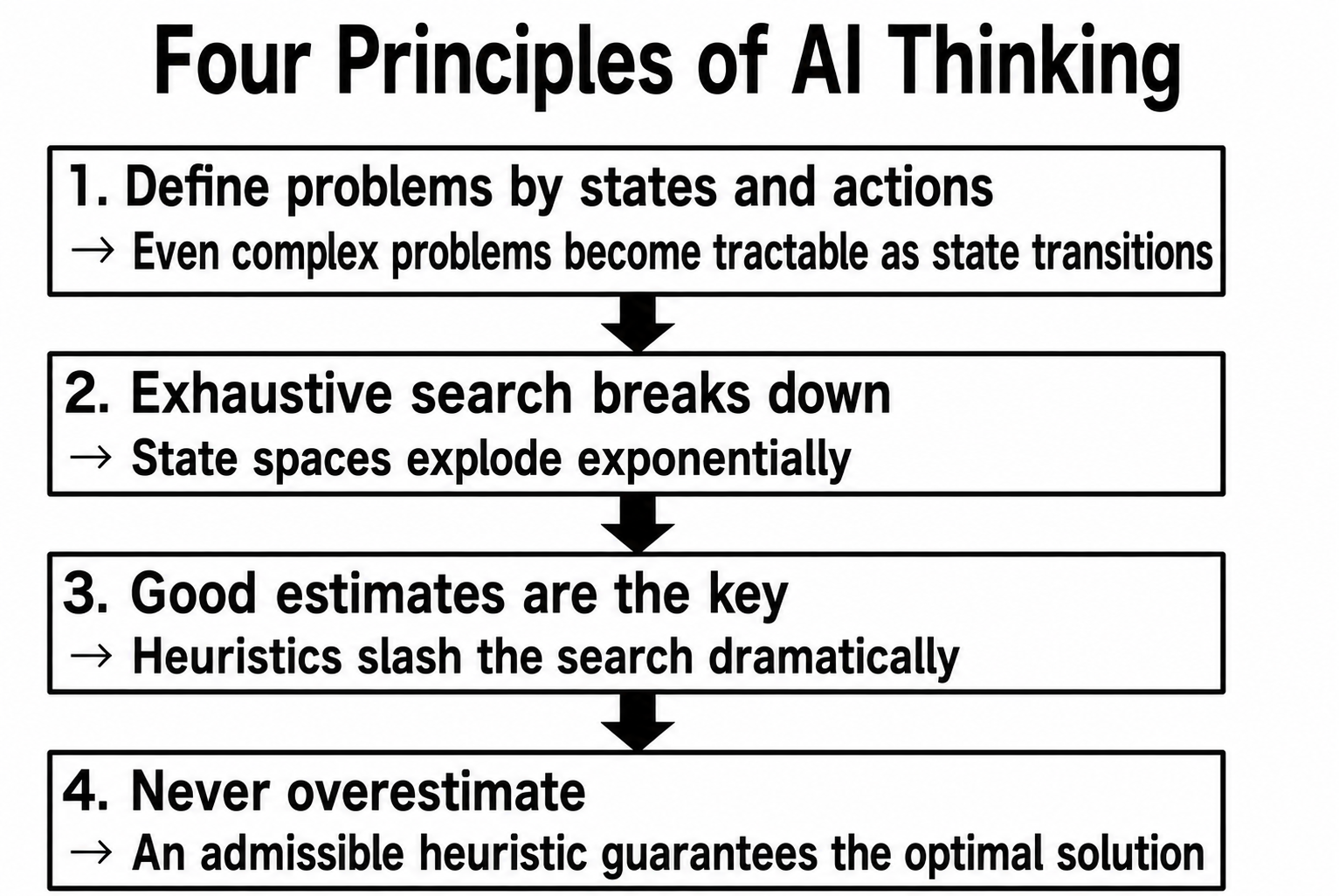
AI is not magic. It is an accumulation of down-to-earth engineering: how to define the states, and how to estimate.
And this basic way of thinking has not changed since the 1960s. Even the newest AI stands on this classical wisdom.
Watch the AI Solve It
Finally, watch the algorithm we have described actually at work.
Scramble the puzzle with "SHUFFLE," then press "AUTO SOLVE" and the AI will solve it one move at a time.
Reading the Statistics
Reading the Statistics
| Item | Description |
|---|---|
| Current depth limit | The threshold IDA* is currently trying. Rises gradually while no solution is found |
| Nodes explored | The number of states actually examined. Grows exponentially with difficulty |
| Solution length | The length of the solution found. This is the shortest path |
| Search time | Time spent computing (milliseconds). Changes dramatically with difficulty |
Change the difficulty and you will see these numbers change dramatically.
Search Volume by Difficulty (Approximate)
| Difficulty | Shuffle | Nodes explored | Search time |
|---|---|---|---|
| Easy | 15 moves | Thousands | A few ms |
| Normal | 30 moves | Tens of thousands | Tens of ms |
| Hard | 50 moves | Hundreds of thousands | Hundreds of ms |
| Expert | 80 moves | Millions | Seconds |
You can see the search volume growing exponentially as difficulty rises.
This is the moment you get to feel the "combinatorial explosion" for yourself.
Code Walkthrough: Implementing IDA* Search
For those interested, here is the actual code. The game uses an algorithm called "IDA* (Iterative Deepening A*)." It uses far less memory than plain A*, which makes it well suited to problems like the 15-puzzle.
What Is IDA*?
IDA stands for "Iterative Deepening A"—that is, A* run with iterative deepening.
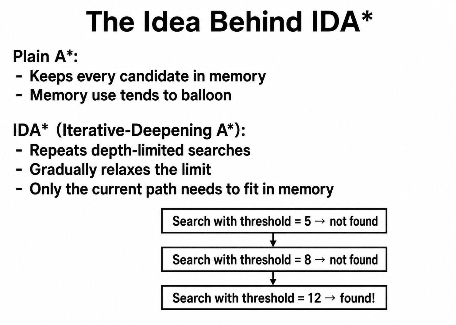
Plain A has one weakness: memory consumption. A must keep every "not yet examined" candidate in memory. In a state space as vast as the 15-puzzle's, memory can run out.
To solve this problem, IDA* adopts the strategy of repeating depth-limited searches.
Why Does This Work So Well?
"Isn't re-exploring the same places wasteful?" you might think. There is indeed some waste. But because the state space grows exponentially, the final iteration accounts for almost all of the total computation time.
Say the solution is found at threshold 10. The searches at thresholds 5, 6, 7, 8, and 9 add up to only a few percent of the search at threshold 10—because search volume grows exponentially as the threshold rises.
In exchange for "a little waste," you gain the huge benefit of "using almost no memory."
Manhattan Distance (the Heuristic Function)
function manhattanDistance(state) {
  let distance = 0;
  for (let i = 0; i < state.length; i++) {
    const tile = state[i];
    if (tile !== 0) {
      // Compute the goal position
      const goalRow = Math.floor(tile / 4);
      const goalCol = tile % 4;
      // Compute the current position
      const currentRow = Math.floor(i / 4);
      const currentCol = i % 4;
      // Add the vertical and horizontal distances
      distance += Math.abs(goalRow - currentRow)
               + Math.abs(goalCol - currentCol);
    }
  }
  return distance;
}
For each tile, compute the vertical and horizontal difference between "where it should be" and "where it is now," and add everything up. The blank (0) is ignored.
The point of this code is that it computes the goal position from the tile's value. For example, tile 5 should sit at index 5 (second row, second column) in the goal state.5 / 4 = 1 (the row) and 5 % 4 = 1 (the column) give you that position.
The IDA* Main Loop
function idaStar(startState) {
  let threshold = manhattanDistance(startState); // initial threshold
  const path = [startState];

  while (true) {
    const result = search(path, 0, threshold);

    if (result === 'FOUND') {
      return path; // solution found
    }

    if (result === Infinity) {
      return null; // no solution
    }

    threshold = result; // raise the threshold and search again
  }
}
IDA* repeats a "depth-limited depth-first search." It first searches with the Manhattan distance as the threshold; if nothing is found, it raises the threshold and tries again.
The important part is how the threshold is updated.search function returns the smallest f(n) value among those that exceeded the threshold, and that becomes the next threshold. This way, the candidates that were "given up on by a hair" get examined in the next iteration.
The Recursive Search
function search(path, g, threshold) {
  const current = path[path.length - 1];
  const f = g + manhattanDistance(current);

  // Cut off if we exceed the threshold
  if (f > threshold) {
    return f;
  }

  // Goal check
  if (isGoal(current)) {
    return 'FOUND';
  }

  let min = Infinity;

  // Explore neighboring states
  for (const neighbor of getNeighbors(current)) {
    path.push(neighbor);
    const result = search(path, g + 1, threshold);

    if (result === 'FOUND') {
      return 'FOUND';
    }

    if (result < min) {
      min = result;
    }

    path.pop(); // backtrack
  }

  return min;
}
f = g + h exceeding the threshold cuts that branch off. This efficiently prunes away states that look far from the goal.
path.pop() is the operation called "backtracking." When "this direction didn't work out," you step back one move and try another. This is why IDA* saves so much memory: instead of holding every candidate, it only needs to keep the current path.
Bonus: Let's Solve the 3×3+1 Picture Puzzle Too!
Here is a bonus for everyone who has read this far.
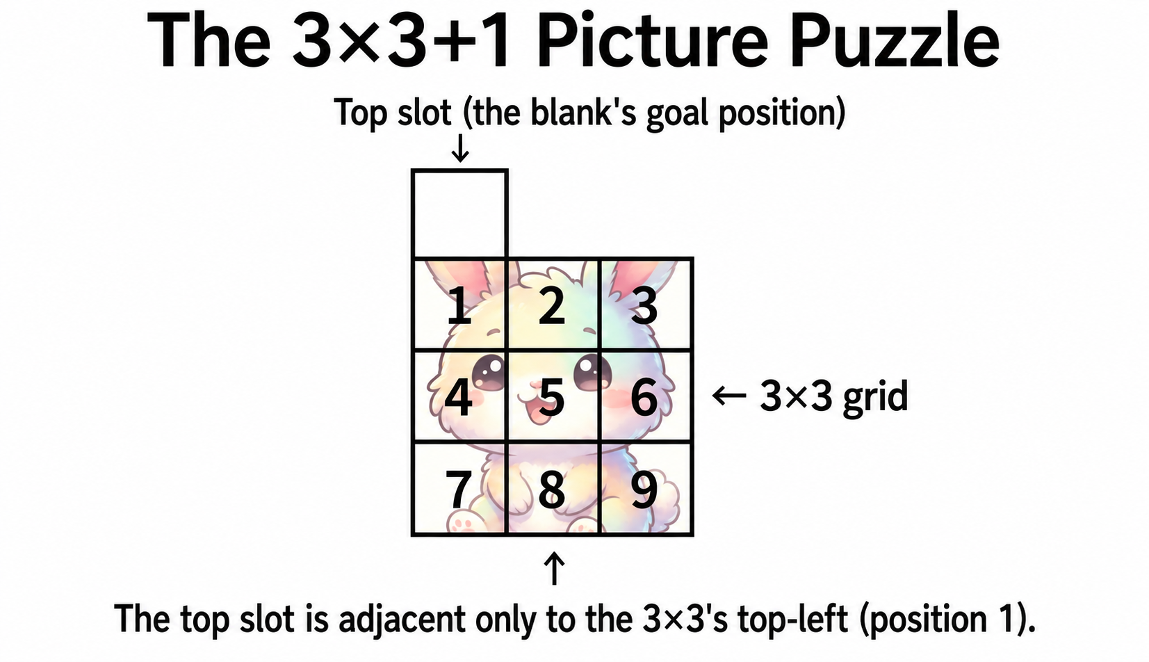
There is another common form of sliding puzzle: the type with a single blank slot on top and a 3×3 picture below. The kind you often see at souvenir shops.
They usually feature cute characters for kids—Disney and the like.
Is the Solution Method the Same?
Yes—basically the same IDA* search solves it!
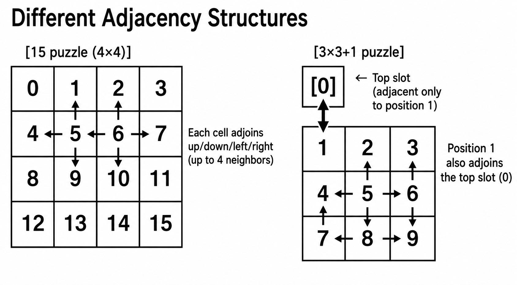
The only difference is the definition of "adjacency."
The Difference in Computation
Comparing state counts
| Puzzle | Squares | States (approx.) |
|---|---|---|
| 3×3+1 | 10 squares | 10!/2 ≈ 1.8 million |
| 15-puzzle | 16 squares | 16!/2 ≈ 10 trillion |
The 3×3+1 puzzle has roughly one five-millionth the states of the 15-puzzle! That is why the search is overwhelmingly faster.
With so few states, the AI's search finishes very quickly on the 3×3+1 puzzle. It is a perfect way to feel the "difference in computational cost" for yourself.
Try It Out
We built a version of this one with the same IDA* search implemented.
Compare the node counts and search times against the 15-puzzle and see how different they are!
The Difference in Code
The algorithm is almost identical; only the definition of adjacency differs.
// Adjacency for the 3×3+1 puzzle
function getAdjacentIndices(index) {
  const adjacency = {
    0: [1],           // top slot → top-left (1) only
    1: [0, 2, 4],     // top-left → top slot, right, down
    2: [1, 3, 5],
    3: [2, 6],
    4: [1, 5, 7],
    5: [2, 4, 6, 8],  // center → up, down, left, right
    6: [3, 5, 9],
    7: [4, 8],
    8: [5, 7, 9],
    9: [6, 8]
  };
  return adjacency[index] || [];
}
In the 15-puzzle we computed "up, down, left, right" arithmetically, but the 3×3+1 puzzle has a special position—the top slot—so we define the adjacency in a table instead.
"Defining adjacency to match the problem's structure" is another important point of state-space search. Even when the problem changes, the skeleton of the algorithm stays the same. What changes are only the "state representation" and the "adjacency."
Closing Thoughts
So there you have it: the humble 15-puzzle sits at the origin of AI research and still connects to today's technology.
What is "thinking"? One answer to that question is "searching a state space." And the trick for searching it smartly was the idea of heuristics.
The next time you come across a 15-puzzle or a picture sliding puzzle, try solving it the way an AI would—
asking yourself, "from the current state, what is the minimum number of moves to the goal?"
That would be a fine first step toward experiencing how an AI "thinks."
Thank you for reading, as always.
See you next time!
Related Articles
The following article, like this one, uses a game to explain another foundation of AI: information theory.
Qualiteg 研究部