Cross-Entropy Explained, Part 2: Classification as Probability and the Likelihood Function

Good morning. This is the Qualiteg Research Department.
Let's pick up right where we left off last time.
Chapter 2: Interpreting Classification as Predicting Probabilities
In the classification problems we want to solve with deep learning, logistic regression, and so on, we predict which class an input belongs to.
First, let's think about what it actually means for an input to be classified as something.
For example, suppose the input is an image of an animal, and consider a classifier that predicts whether that image shows a dog, a fox, or a wolf.
(Think of the classifier as program code with an input, a process, and an output: the input is image data, the process is a computation such as a neural network or logistic regression, and the output is the classification result.)
If we feed this classifier an image of a dog, for instance, the result is not a direct verdict of "dog."
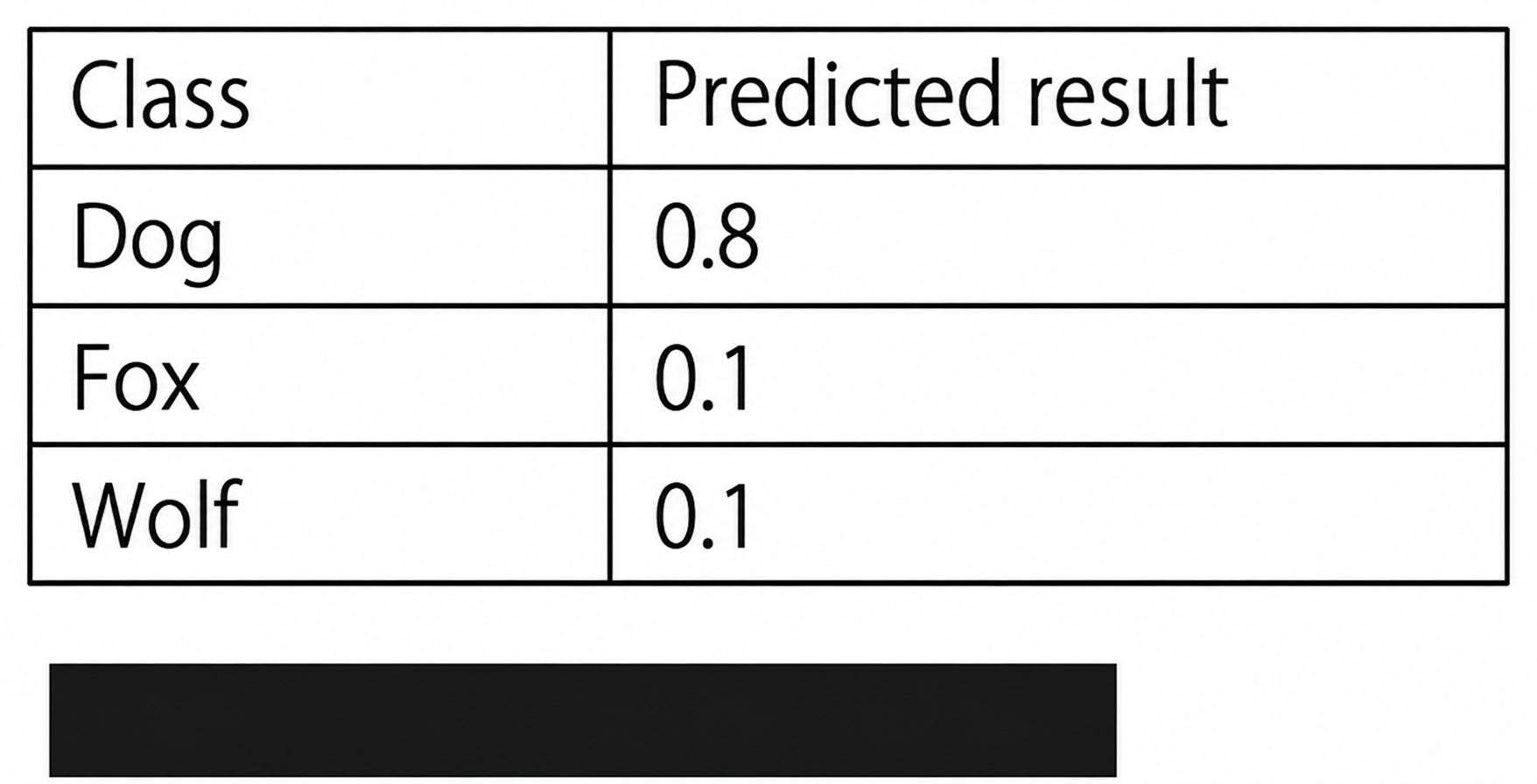
Instead, the classification takes the form of predicted probability values, like this: a probability of 0.8 that it is a "dog," 0.1 that it is a "fox," and 0.1 that it is a "wolf."
With this in mind, namely that a classification problem is a prediction of probability values, let's now look at cross-entropy.
Chapter 3: Dice Rolls and the Likelihood Function
As noted above, classification is a prediction of probability values, so from here on we will use the concept of probability to derive cross-entropy.
Here we have a die.
It is not an ordinary die; it seems to have been tampered with somehow.
In other words, it is a loaded die, so the outcomes are biased. That is our setup.
3-1. Events
Let's consider the events that occur when we roll the die. An event is something that happens. When we roll a die, the event that occurs is, in the end, that some face comes up.
Since it is a die, there are six possible events when it is rolled, as follows.
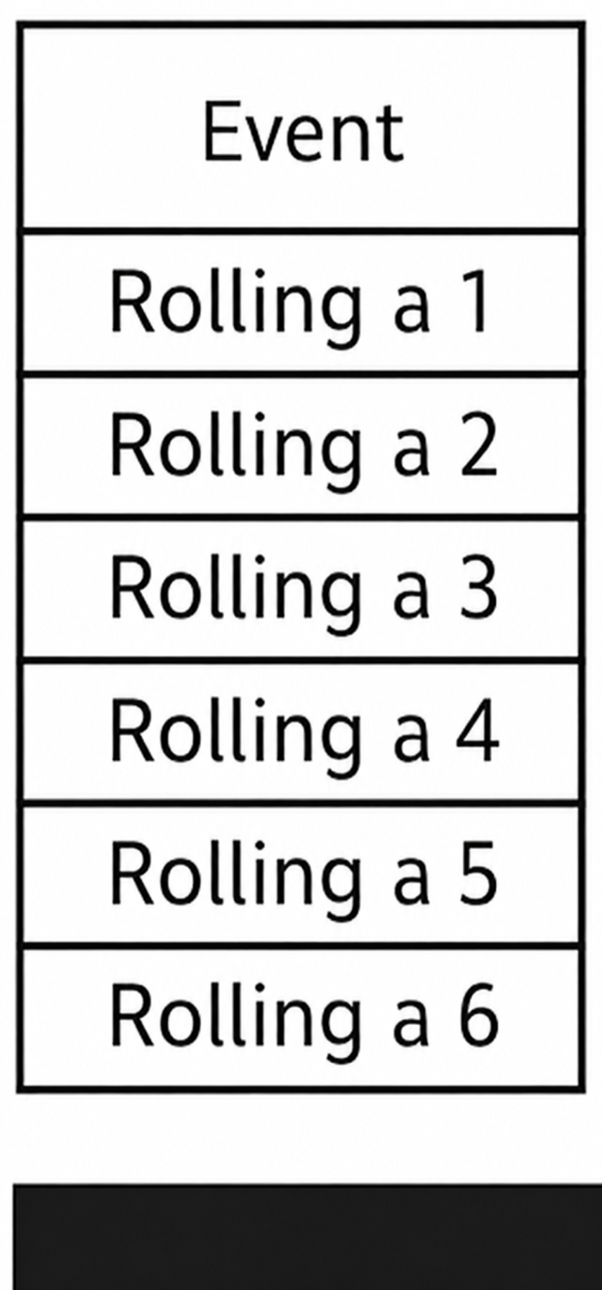
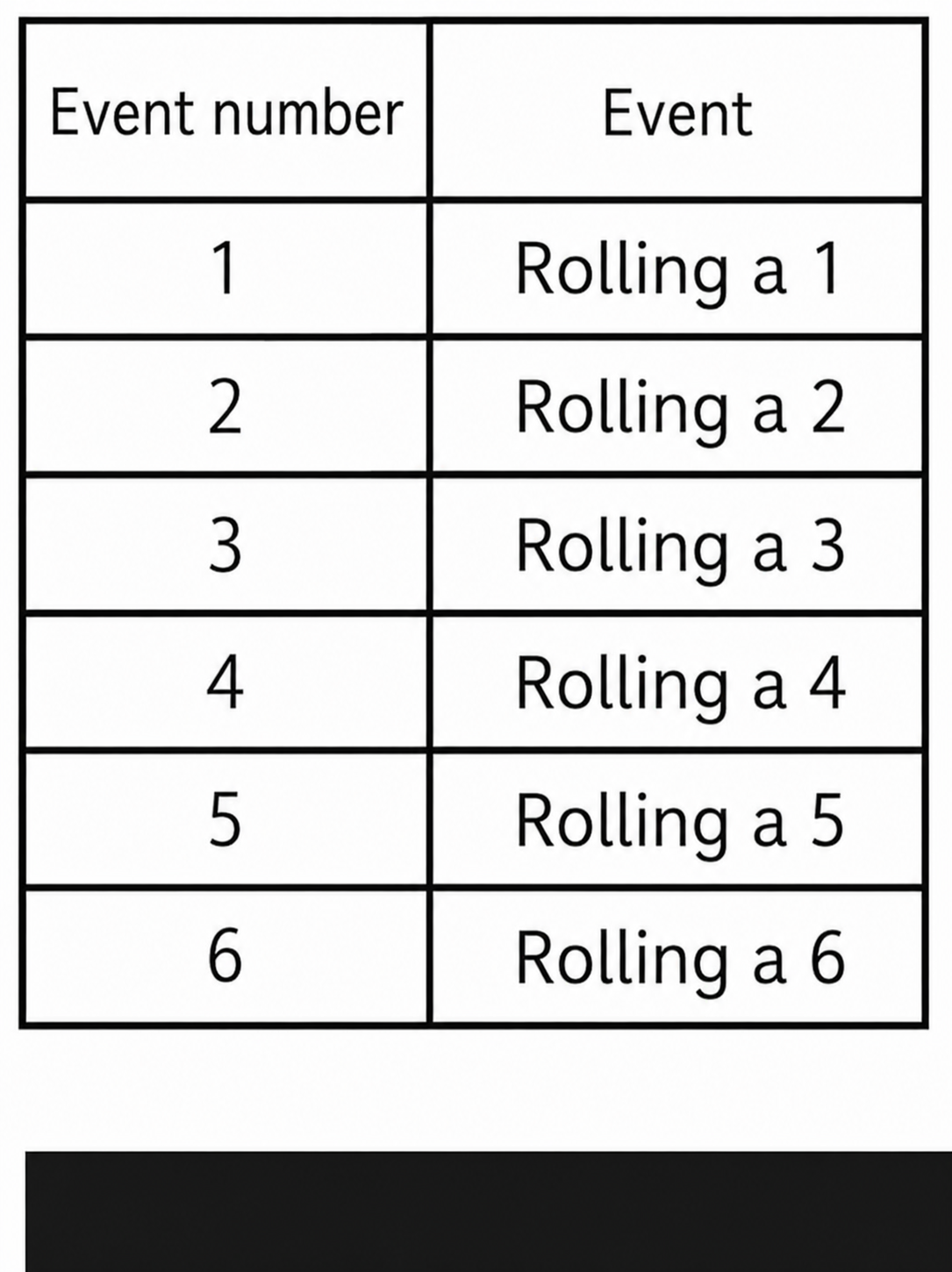
From here on, we will number these six events and refer to them as "event \(_1\)", "event \(_2\)", "event \(_3\)", and so on.
3-2. The probability of a given face coming up
From here, let's think about how to actually roll the die, tally the outcomes, and estimate "which face comes up, and with what probability."
With a fair die, every face comes up with probability \(\frac{1}{6}\). As mentioned above, however, our setup uses a tampered, loaded die, so we cannot predict in advance which face comes up with what probability.
What we want to know, then, is the probability of each face of this die coming up, so we add the probability that each event occurs to the table as follows.
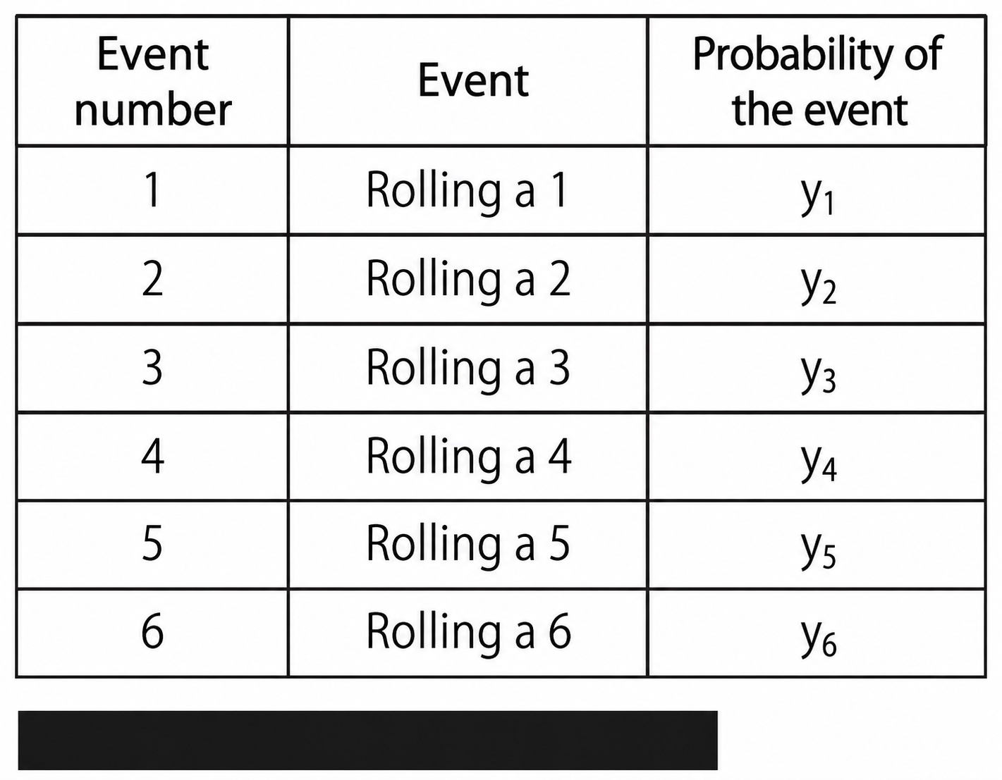

We set the variables \(y1\) through \(y6\) as follows: the probability that a 1 comes up is \(y1\), the probability that a 2 comes up is \(y2\), and so on.
When we roll the die, one of the faces \(1\) through \(6\) comes up, so the sum of the probabilities that the events occur (that is, the probability that some face comes up) is naturally \(1\).
$$
y_{1} + y_{2} + y_{3} + y_{4} + y_{5} + y_{6} = 1 \tag{3.1}
$$
Rewriting this with \(\sum\) gives the following.
$$
L = \sum_{i=1}^{6} y_i = 1 \tag{3.2}
$$
3-3. Actually rolling the die
Now let's roll the die and see which faces come up.
Suppose the results of rolling this die 20 times were as follows.
(At a glance, it looks like a die that tends to land on even numbers.)
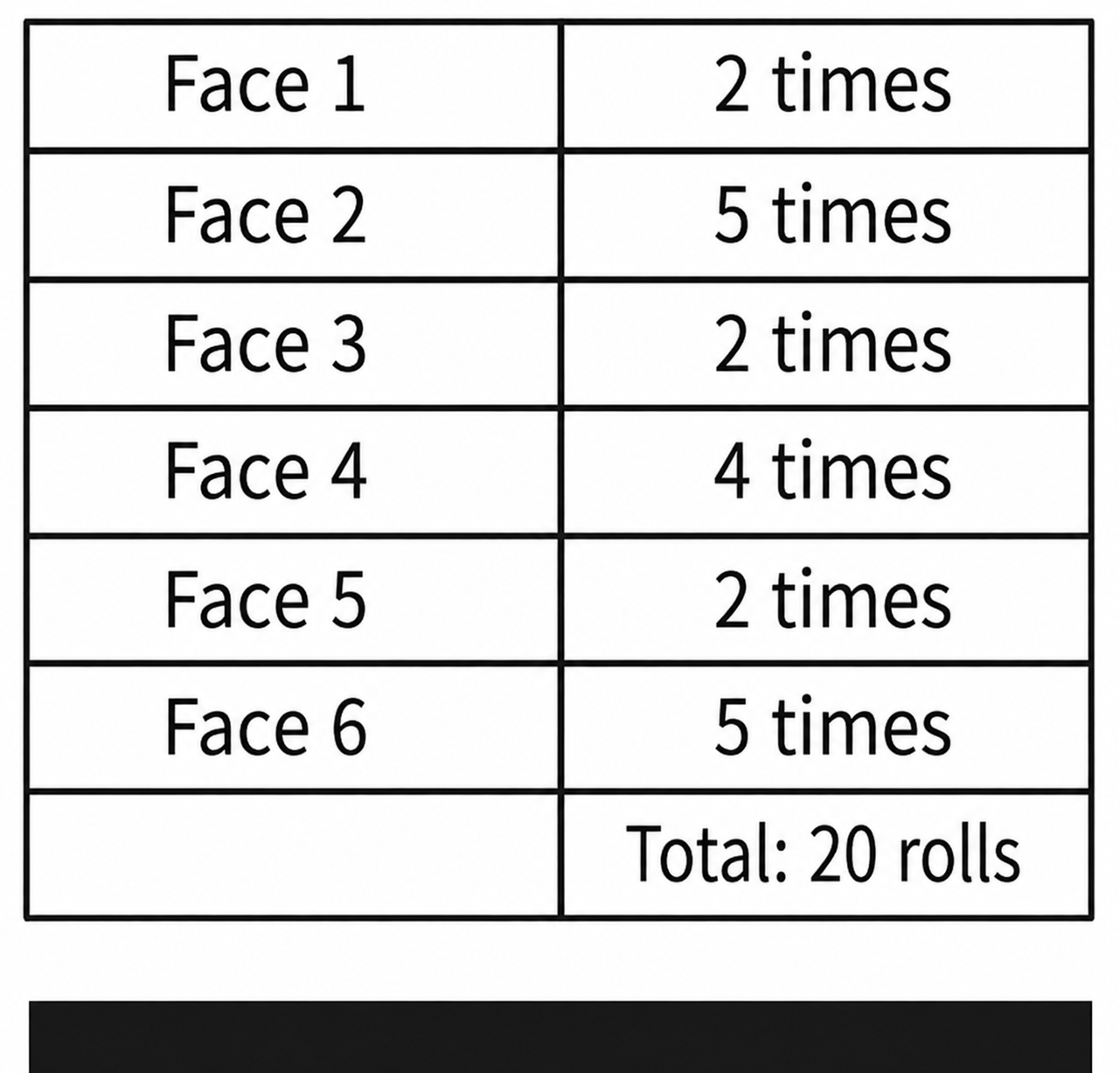
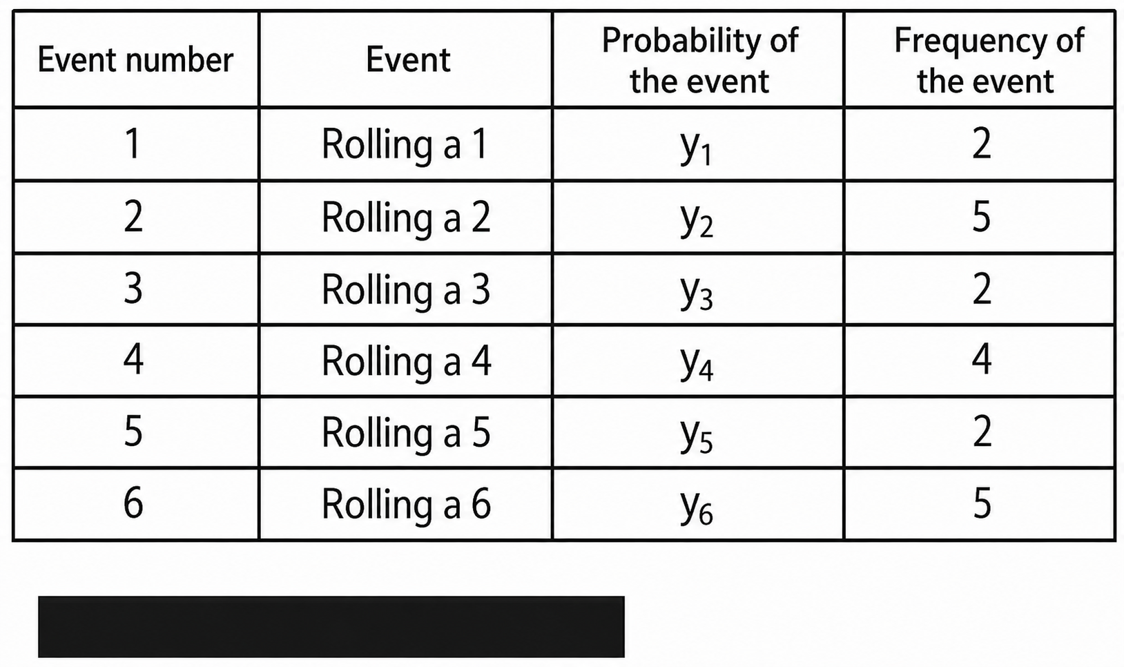
After 20 rolls, we now know how often each event occurred: a 1 came up twice, a 2 came up five times, and so on. So we add a column for the frequency of each event to the earlier table, as shown below.
3-4. The likelihood function
Now let's use what we have organized so far to compute probabilities.
If we replace the frequency of each event in the table above with a variable \(t\), and attach the event number as a subscript to write it as \(t_{1}\) through \(t_{6}\), we get the following.
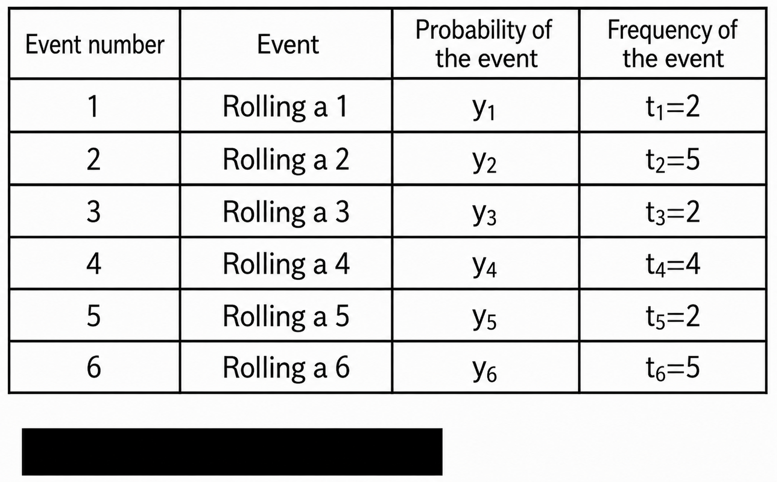
What is the probability that rolling the die 20 times gives the results in the table above?
Each roll of the die is an independent trial (the result of the second roll is not affected by the first), so since a 1 came up 2 times, a 2 came up 5 times, a 3 came up 2 times, a 4 came up 4 times, a 5 came up 2 times, and a 6 came up 5 times, the probability is
$$
y_{1} \times y_{1} \times y_{2} \times y_{2} \times y_{2} \times y_{2} \times y_{2} \times y_{3} \times y_{3} \times y_{4} \times y_{4} \times y_{4} \times y_{4} \times y_{5} \times y_{5} \times y_{6} \times y_{6} \times y_{6} \times y_{6} \times y_{6}
$$
Rewriting this in exponent notation, using the event frequencies \(t_{1}\) through \(t_{6}\) as the exponents, gives
$$
y_{1}^{t_{1}} \cdot y_{2}^{t_{2}} \cdot y_{3}^{t_{3}} \cdot y_{4}^{t_{4}} \cdot y_{5}^{t_{5}} \cdot y_{6}^{t_{6}}
$$
(We also replaced \(\times\) with \(\cdot\) while we were at it.)
This expression \(y_{1}^{t_{1}} \cdot y_{2}^{t_{2}} \cdot y_{3}^{t_{3}} \cdot y_{4}^{t_{4}} \cdot y_{5}^{t_{5}} \cdot y_{6}^{t_{6}}\), which contains the probabilities \(y_{1}\) through \(y_{6}\) that events \(1\) through \(6\) occur when the die is rolled, is called the likelihood function (or simply the likelihood).
Using \(L\) for likelihood, the likelihood function is written as follows.
$$
L = y_{1}^{t_{1}} \cdot y_{2}^{t_{2}} \cdot y_{3}^{t_{3}} \cdot y_{4}^{t_{4}} \cdot y_{5}^{t_{5}} \cdot y_{6}^{t_{6}} \tag{3.3}
$$
If we denote the event number in the subscript of \(y\) by \(i\) and write the product with the product symbol \(\prod\), we get the following.
(\(\prod\) is the multiplication counterpart of \(\sum\).)
$$
L = \prod_{k=1}^{6} y_k^{t_{k}} \tag{3.4}
$$
Let's recall the original question here.
We wanted a method to "estimate which face comes up, and with what probability, since this loaded die has biased outcomes."
One such method is maximum likelihood estimation (the maximum likelihood method).
The problem maximum likelihood estimation poses is: "What plausible values of \(y_{1}\) through \(y_{6}\) best explain the results of these 20 trials?"
Put another way:
"What values of \(y_{1}\) through \(y_{6}\) would produce results like those of these 20 trials?"
In other words, we want to find the plausible parameters \({y_{1}}\), \({y_{2}}\), \({y_{3}}\), \({y_{4}}\), \({y_{5}}\), \({y_{6}}\) that maximize the likelihood function \(L\) above.
3-5. Maximum likelihood estimation
We have now framed the problem as "find the parameters \({y_{1}}\), \({y_{2}}\), \({y_{3}}\), \({y_{4}}\), \({y_{5}}\), \({y_{6}}\) that maximize the likelihood function \(L\)." But how do we maximize the likelihood function \(L\)?
One way to find the maximum of a function is to differentiate it and find where the derivative equals \(0\).
When you differentiate a function, the resulting function (the derivative) represents the slope of the tangent to the original function, so the point where that slope is \(0\) is where the original function takes its maximum.
(More precisely, a point where the tangent slope is \(0\) is a local maximum or local minimum of the original function. We will explain in a supplement that, by examining the second derivative of the likelihood function (differentiating it twice), the point where the slope is \(0\) is indeed a maximum.)
Finding the parameters that maximize the likelihood function \(L\) in this way (the maximum likelihood estimates) is called maximum likelihood estimation (the maximum likelihood method).
3-6. The log-likelihood function
To find the maximum of the likelihood function, we need to find the point where its derivative is \(0\), so we want to differentiate the likelihood function \(L\). However, the likelihood function is a product, as shown below, which makes it awkward to differentiate as it stands. Furthermore, when we later compute it on a computer, we would be multiplying probability values (between \(0\) and \(1\)) over and over, so the result becomes extremely small, which can be a problem given the numerical precision of computers.
So instead we consider the log-likelihood function \(log L\), obtained by taking the logarithm of the likelihood function \(L\) as follows.
Taking the logarithm \(log\) has the effect of turning multiplication into addition, which makes differentiation and computation easier.
Expanding once more the likelihood function \(L\) that we wrote earlier using \(\prod\),
$$
\begin{aligned}
L &= \prod_{k=1}^{6} y_k^{t_{k}}& \
&= y_{1}^{t_{1}} \cdot y_{2}^{t_{2}} \cdot y_{3}^{t_{3}} \cdot y_{4}^{t_{4}} \cdot y_{5}^{t_{5}} \cdot y_{6}^{t_{6}}&
\end{aligned}
$$
we take its logarithm to get the form \(log L\) below.
Because it is the logarithm of the likelihood function, it is called the log-likelihood function.
$$
\log L = \log (y_{1}^{t_{1}} \cdot y_{2}^{t_{2}} \cdot y_{3}^{t_{3}} \cdot y_{4}^{t_{4}} \cdot y_{5}^{t_{5}} \cdot y_{6}^{t_{6}}) \tag{3.5}
$$
Logarithm rules
Let's briefly recall the rules of logarithms here.
Logarithm rule 1
$$
\log ab = \log a + \log b
$$
Logarithm rule 2
$$
\log a^{b} = b \log a
$$
With these rules in mind, let's transform equation (\(3.5\)).
$$
\begin{aligned}
\log L =&\log (y_{1}^{t_{1}} \cdot y_{2}^{t_{2}} \cdot y_{3}^{t_{3}} \cdot y_{4}^{t_{4}} \cdot y_{5}^{t_{5}} \cdot y_{6}^{t_{6}})& \
\
&\text{By logarithm rule 1, turn the product inside } \log \text{ into a sum}&\\
=&\log y_{1}^{t_{1}} + \log y_{2}^{t_{2}} + \log y_{3}^{t_{3}} + \log y_{4}^{t_{4}} + \log y_{5}^{t_{5}} + \log y_{6}^{t_{6}}&\
\\
&\text{By logarithm rule 2, bring the exponents down}&\\
=&t_{1} \log y_{1} + t_{2} \log y_{2} + t_{3} \log y_{3} + t_{4} \log y_{4} + t_{5} \log y_{5} + t_{6} \log y_{6} &\
\
\end{aligned}
$$
By taking the logarithm, we have arrived at a form that is much easier to handle.
$$
\begin{aligned}
\log L=&t_{1} \log y_{1} + t_{2} \log y_{2} + t_{3} \log y_{3} + t_{4} \log y_{4} + t_{5} \log y_{5} + t_{6} \log y_{6} &
\end{aligned}
$$
Furthermore, replacing the subscripts \(1\) through \(6\) with \(k\) and writing it with \(\sum\) gives the following.
$$
\log L=\sum_{k=1}^{6} t_{k} \log y_{k} \tag{3.6}
$$
So far, the log-likelihood function for the outcomes of 20 rolls of the die has come out as follows.
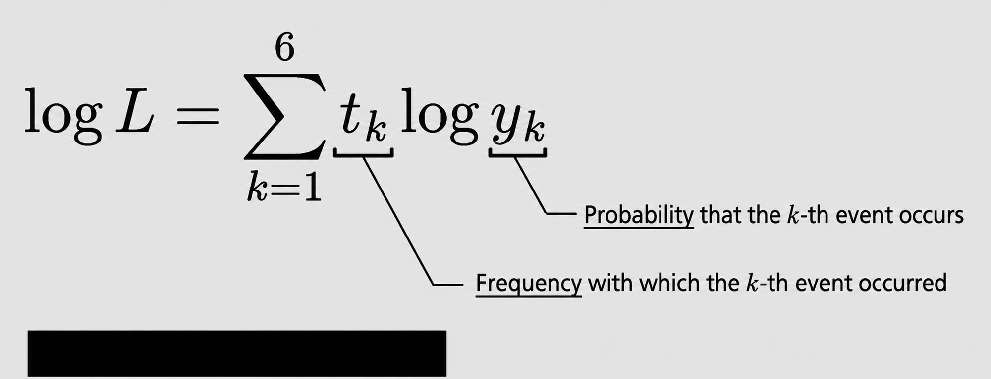
You may be wondering where the number of trials, 20, went. It is reflected in the sum of the frequencies \(t_{k}\), that is, in \(\sum_{k=1}^{6}t_{k}\).
$$
\sum_{k=1}^{6}t_{k} = 20
$$
Summary
How was that?
This time, starting from the idea of viewing classification problems through the lens of probability, we studied a concrete probability problem: estimating the outcomes of a die. With an ordinary die every face comes up with equal probability, but as a special case we used a loaded die biased toward certain faces.
We built a "likelihood function" that uses variables to express how often each face comes up when such a biased die is rolled, and to think about how to estimate the probability of each face using it, we introduced the technique of "maximum likelihood estimation."
Furthermore, to make this estimation method easier to work with, we introduced the "log-likelihood function" by taking the logarithm of the likelihood function, turning it into a simpler, clearer form that is mathematically (and computationally) easier to handle.
Through this process, we walked through the concrete steps of how probabilities are actually computed, starting from the rolls of a biased die.
Next time, we will derive cross-entropy from the likelihood function.
See you next time.
References
https://journal.qualiteg.com/books/
navigation