Cross-Entropy Explained, Part 4: Cross-Entropy for Multi-Class Classification (Single Sample)

Good morning! This is the Research Department at Qualiteg Inc.

In this installment, we will calculate the cross-entropy used for multi-class classification.

Chapter 5: Calculating Cross-Entropy for Multi-Class Classification (Single-Sample Version)

First, let us restate the cross-entropy function (single-sample version).

$$
\ - \log L=\sum_{k=1}^{K} t_{k} \log y_{k} \tag{4.3, restated}
$$

$$
t_{k} :\text{frequency}, y_{k}:\text{probability}
$$

The cross-entropy in equation \((4.3)\) covered a single sample containing \(K\) events (each of which either occurred or did not occur).

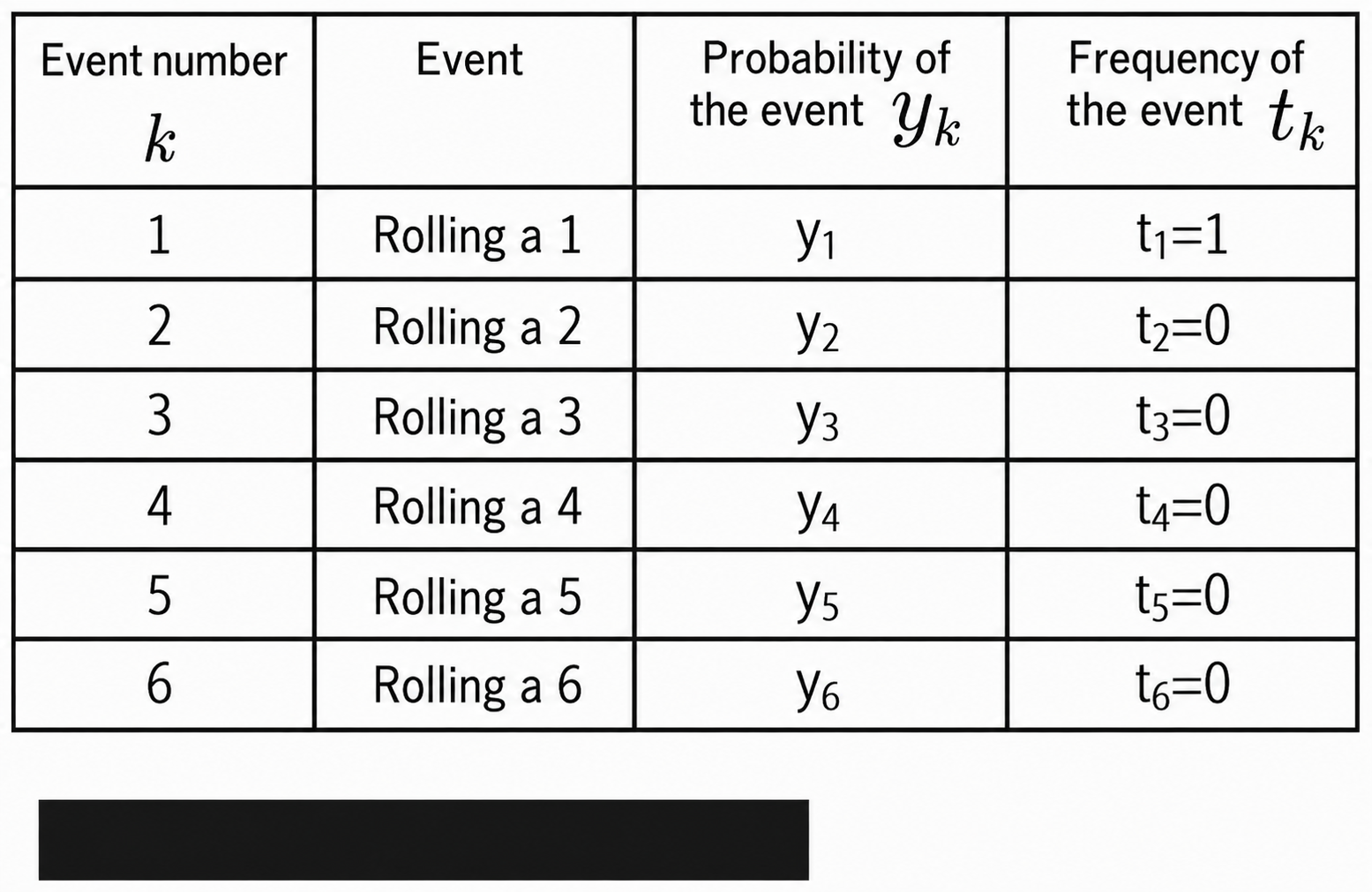
In the dice example, this means that a single roll has \(K=6\) possible outcomes. The variables were \(y_{k} :\) probability and \(t_{k} :\) frequency.

Now, building on what we have covered so far,
let us switch our mindset from probability to classification problems.

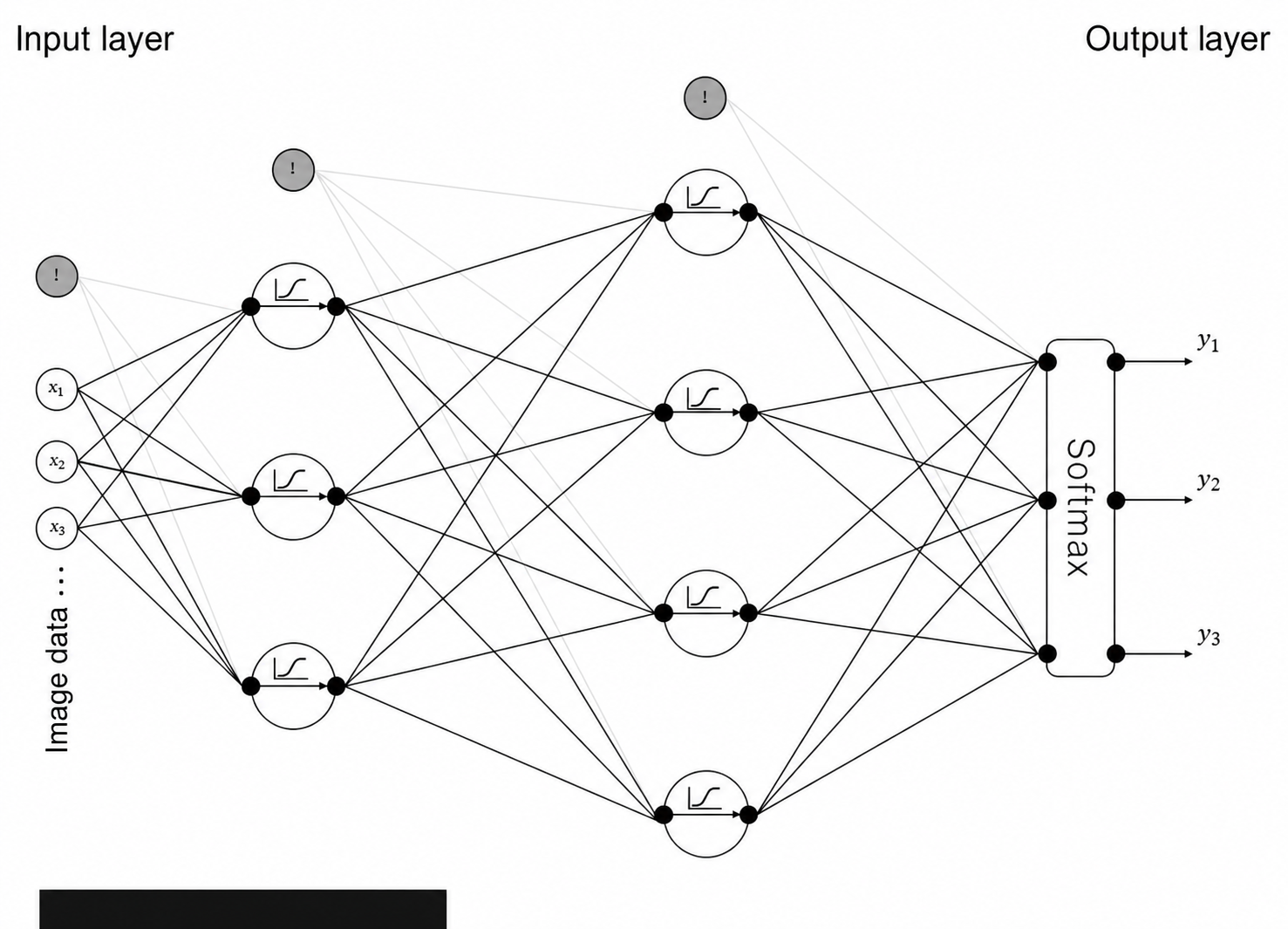
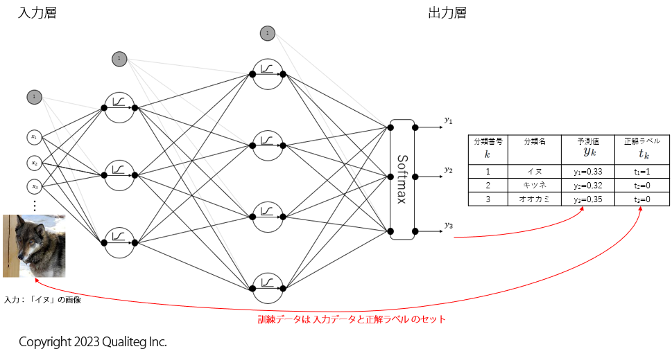
Consider a neural network model like the one below. (The details of the model are not important.)

Given an image as input, this model predicts the probability that the image is a "dog", the probability that it is a "fox", and the probability that it is a "wolf".

Assume that this model has not been trained at all yet.

In this state, we fed it an image of a "dog" just to see what happens, and got the following result.

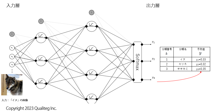
Since the model has not been trained, its predictions are still far from correct, but the predicted value \(y_{1}\) for "dog" came out as \(0.33\), the predicted value \(y_{2}\) for "fox" as \(0.32\), and the predicted value \(y_{3}\) for "wolf" as \(0.35\).

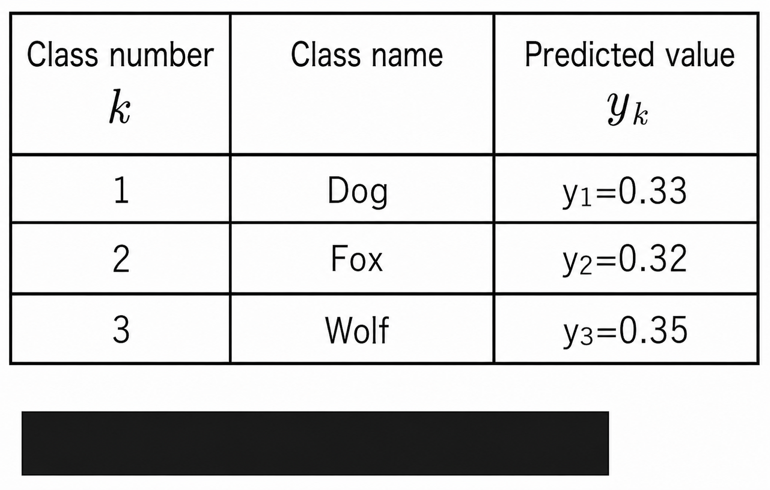
Now, let us consider the probability \(L\) that the model's predictions are correct. In this example, we already know that "dog" is the correct answer and that "fox" and "wolf" are incorrect, so we can compute

$$
\begin{aligned}
L = &y_{1}^{1} \cdot y_{2}^{0} \cdot y_{3}^{0}&
\
=&0.33^{1} \times 0.32^{0} \times 0.35^{0}&\
=&0.33&
\end{aligned}
$$

(At \(0.33\) it is still a poor model, but this is what the calculation gives.)

If we assign \(1\) to "dog" because it is correct, and \(0\) to "fox" and "wolf" because they are incorrect, the correct/incorrect answers can be organized as a column of ground-truth labels \(t_{k}\), as shown below.

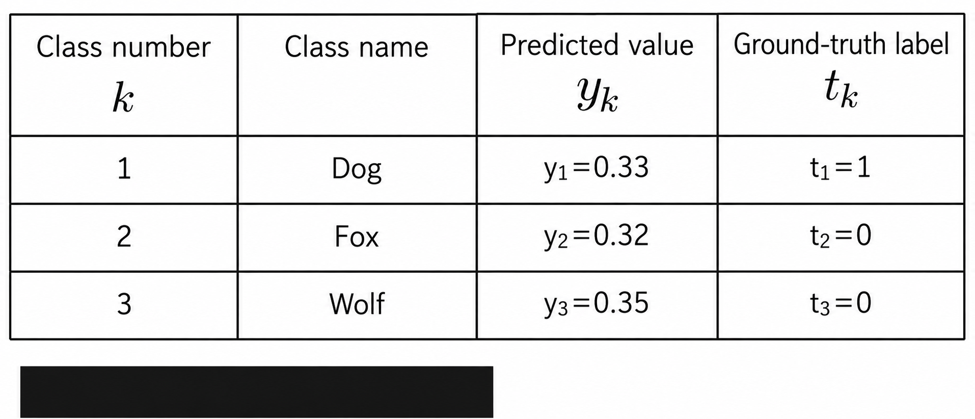
Expressing the probability \(L\) in terms of \(y_{k}\) and \(t_{k}\), we get

$$
\begin{aligned}
L = &y_{1}^{t_{1}} \cdot y_{2}^{t_{2}} \cdot y_{3}^{t_{3}}&
\
=&\prod_{k=1}^3 y_{k}^{t_{k}} &\
\end{aligned}
$$

This is the same formula as the likelihood per single trial in the dice example, so here too we will treat the probability derived by this calculation as the likelihood.

Also as in the dice example, taking the logarithm of the probability \(L\) and rearranging the expression for the log-likelihood gives

$$
\begin{aligned}
\log L =&\log (y_{1}^{t_{1}} \cdot y_{2}^{t_{2}} \cdot y_{3}^{t_{3}}) & \
\
&\text{By logarithm rule (1): } \log ab = \log a + \log b&\\
=&\log y_{1}^{t_{1}} + \log y_{2}^{t_{2}} + \log y_{3}^{t_{3}}&\
\\
&\text{By logarithm rule (2): } \log a^{b} = b \log a&\\
=&t_{1} \log y_{1} + t_{2} \log y_{2} + t_{3} \log y_{3}&\
\
=&\sum_{k=1}^{3} t_{k} \log y_{k}&\
\
&t_{k}:\text{ground-truth label}, y_{k}:\text{predicted value}&
\end{aligned}
$$

This time we had three classes, "dog", "fox", and "wolf", but if we replace the subscripts \(1\) to \(3\) with \(K\) and write it using \(\sum\), we get the following.

$$
\log L = \sum_{k=1}^{K} t_{k} \log y_{k} \tag{5.1} \
$$

$$
\begin{aligned}
&K:\text{number of classes},\ t_{k}:\text{ground-truth label},\ y_{k}:\text{predicted value}&
\end{aligned}
$$

This is the log-likelihood function.

As we already confirmed in the dice example, the cross-entropy \(E\) is the negative of the log-likelihood function, so

$$
E = - \log L
$$

$$
E = - \sum_{k=1}^{K} t_{k} \log y_{k} \tag{5.2}
$$

$$
\begin{aligned}
&K:\text{number of classes},\ t_{k}:\text{ground-truth label},\ y_{k}:\text{predicted value computed by the model}&
\end{aligned}
$$

We have now defined the cross-entropy function \(E\) per single training sample used during training.

Let us immediately use the data below once more with the cross-entropy function \(E\) in equation \((5.2)\) to calculate the cross-entropy error for a single training sample.

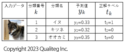
$$
\begin{aligned}
\ E = &- \sum_{k=1}^{K} t_{k} \log y_{k} &\
&= - ( t_{1} \log y_{1} + t_{2} \log y_{2} + t_{3} \log y_{3}) & \
&= - ( 1 \cdot \log 0.33 + 0 \cdot \log 0.32 + 0 \cdot \log 0.35) \
&= -0.481486 \
\
&K:\text{number of classes},\ t_{k}:\text{ground-truth label},\ y_{k}:\text{predicted value computed by the model}&
\end{aligned}
$$

Using this cross-entropy error as the loss function and updating the model's weight parameters so that the loss becomes smaller is the basic form of neural network training.

Incidentally, what we have here is the loss function used for training on a single training sample, as shown below. From the result \(y_{k}\) obtained by feeding one input sample into the neural network and the ground-truth label \(t_{k}\), we calculated the cross-entropy error as the error function.

In this installment, we calculated the cross-entropy for multi-class classification in the single-sample case.

Next time, we will extend this to N samples.

See you next time!

References
https://journal.qualiteg.com/books/

navigation