Cross-Entropy Explained, Part 6: Cross-Entropy for Binary Classification

Good morning from the Qualiteg Research Team.

This time, let's look at cross-entropy for binary classification.

Chapter 7: Cross-Entropy for Binary Classification

7-1. Cross-Entropy for Binary Classification (Single-Sample Version)

From here, we would like to derive the cross-entropy for binary classification.

Binary classification predicts which of two classes the input data belongs to.

To keep things simple, let's first recall the single-sample (non-batch) cross-entropy formula given in Equation \((5.2)\).

$$
E = - \sum_{k=1}^{K} t_{k} \log y_{k} \tag{5.2, restated}
$$

$$
\begin{aligned}
&K:\text{number of classes},　t_{k}:\text{ground-truth label},　y_{k}:\text{predicted value computed by the model}&
\end{aligned}
$$

If we regard binary classification as a special case of multi-class classification, Equation \((5.2)\) should work as is.

That is, for multi-class classification we have \(K \ge 3 \), whereas for binary classification the number of classes is 2, so \(K=2\).

So, letting \(BCE\) denote the cross-entropy when \(K=2\), and expanding Equation \((5.2)\), we get the following.

(BCE is short for Binary Cross Entropy, i.e., cross-entropy for binary classification.)

$$
\begin{aligned}
\ BCE = &- \log L&\
\ = &- \sum_{k=1}^{2} t_{k} \log y_{k}&\
\ = &- (t_{1} \log y_{1} + t_{2} \log y_{2} ) &\
\end{aligned}
$$

That gives us:

$$
\ BCE =- (t_{1} \log y_{1} + t_{2} \log y_{2} ) \tag{7.1}
$$

As binary classification data, let's consider the classification problem introduced at the beginning of this series: predicting whether a passenger on the Titanic survived or did not survive.

The data source is as follows.

Author: Frank E. Harrell Jr., Thomas Cason
Source:?Vanderbilt Biostatistics
(http://biostat.mc.vanderbilt.edu/wiki/pub/Main/DataSets/titanic.html)

First, suppose the data for a passenger who "survived" and the model's predicted values are as follows.

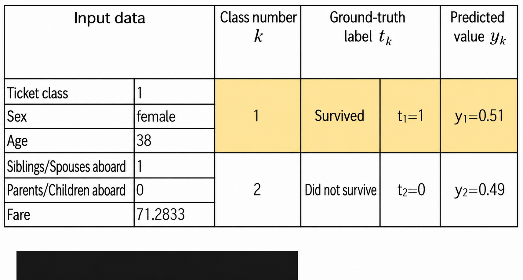
Computing the cross-entropy \(BCE\) gives:

$$
\begin{aligned}
\ \ BCE =&- (t_{1} \log y_{1} + t_{2} \log y_{2} )&\
=&- (1 \cdot \log 0.51 + 0 \cdot \log 0.49 )&\
=&- \log 0.51&\
\end{aligned}
$$

Similarly, let's now compute the cross-entropy for the following data representing a passenger who "did not survive."

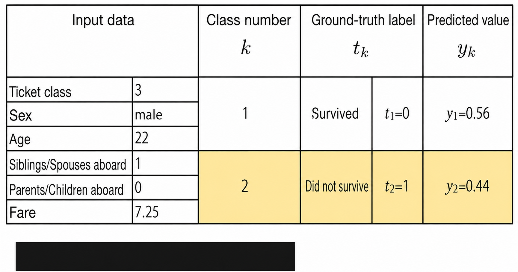
$$
\begin{aligned}
\ \ BCE =&- (t_{1} \log y_{1} + t_{2} \log y_{2} )&\
=&- (0 \cdot \log 0.56 + 1 \cdot \log 0.44 )&\
=&- \log 0.44&\
\end{aligned}
$$

As you can see, it is of course possible to compute the cross-entropy for binary classification using the multi-class approach.

Now, in classification problems where we compute probabilities, the predicted values sum to 1.

Also, since the ground-truth label is 1 for the correct class and 0 otherwise, the labels also sum to 1.

In other words, for a binary problem,

$$
y_{1} + y_{2} = 1
$$

$$
t_{1} + t_{2} = 1
$$

and therefore

$$
y_{2} = 1-y_{1}
$$

$$
t_{2} = 1-t_{1}
$$

Substituting these into the cross-entropy formula for \(K=2\) shown in Equation \((7.1)\), \(BCE =- (t_{1} \log y_{1} + t_{2} \log y_{2})\), we get

$$
\begin{aligned}
BCE =&- (t_{1} \log y_{1} + t_{2} \log y_{2} )&\
=&- (t_{1} \log y_{1} + (1-t_{1}) \log (1-y_{1}) )&
\end{aligned}
$$

which means the formula can be rewritten using only \(t_{1}\) and \({y_{1}}\).

$$
BCE=- (t_{1} \log y_{1} + (1-t_{1}) \log (1-y_{1}) ) \tag{7.2}
$$

As Equation \((7.2)\) shows,
for a single data sample, the ground-truth label and predicted value are now just \(t_{1}\) and \(y_{1}\).
( \(t_{2}\) and \(y_{2}\) have disappeared as a result of the rewrite.)

Since there is no longer any need to attach the subscript " \({1}\) " as in ground-truth label \(t{1}\) and predicted value \(y_{1}\), we drop the subscript and write the ground-truth label and predicted value as \(t\) and \(y\).

The resulting Equation \((7.3)\) is the cross-entropy function for binary classification (for a single data sample).

$$
BCE=- (t \log y + (1-t) \log (1-y) ) \tag{7.3}
$$

$$
t:\text{ground-truth label}\quad y:\text{predicted value}
$$

For a binary classification model that uses \((7.3)\) as its loss function, the input data, ground-truth label, and predicted value look like the following.

This input data corresponds to a passenger aboard the Titanic who "survived," so it is given the ground-truth label \(t=1\).

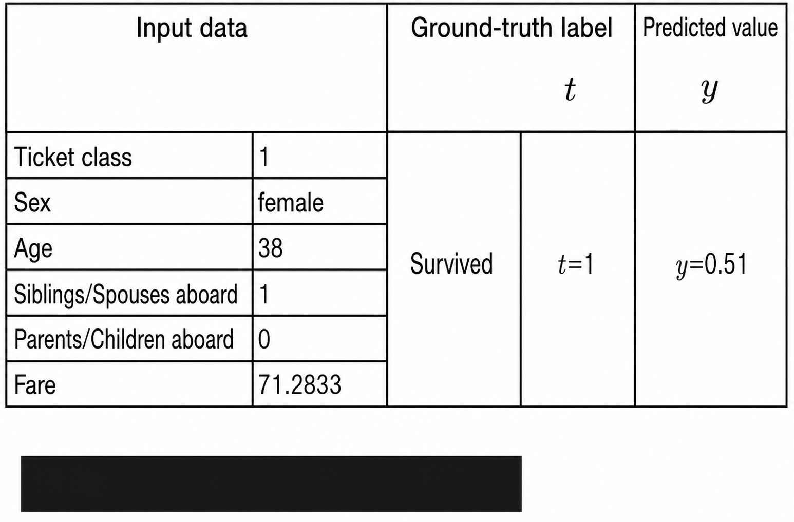
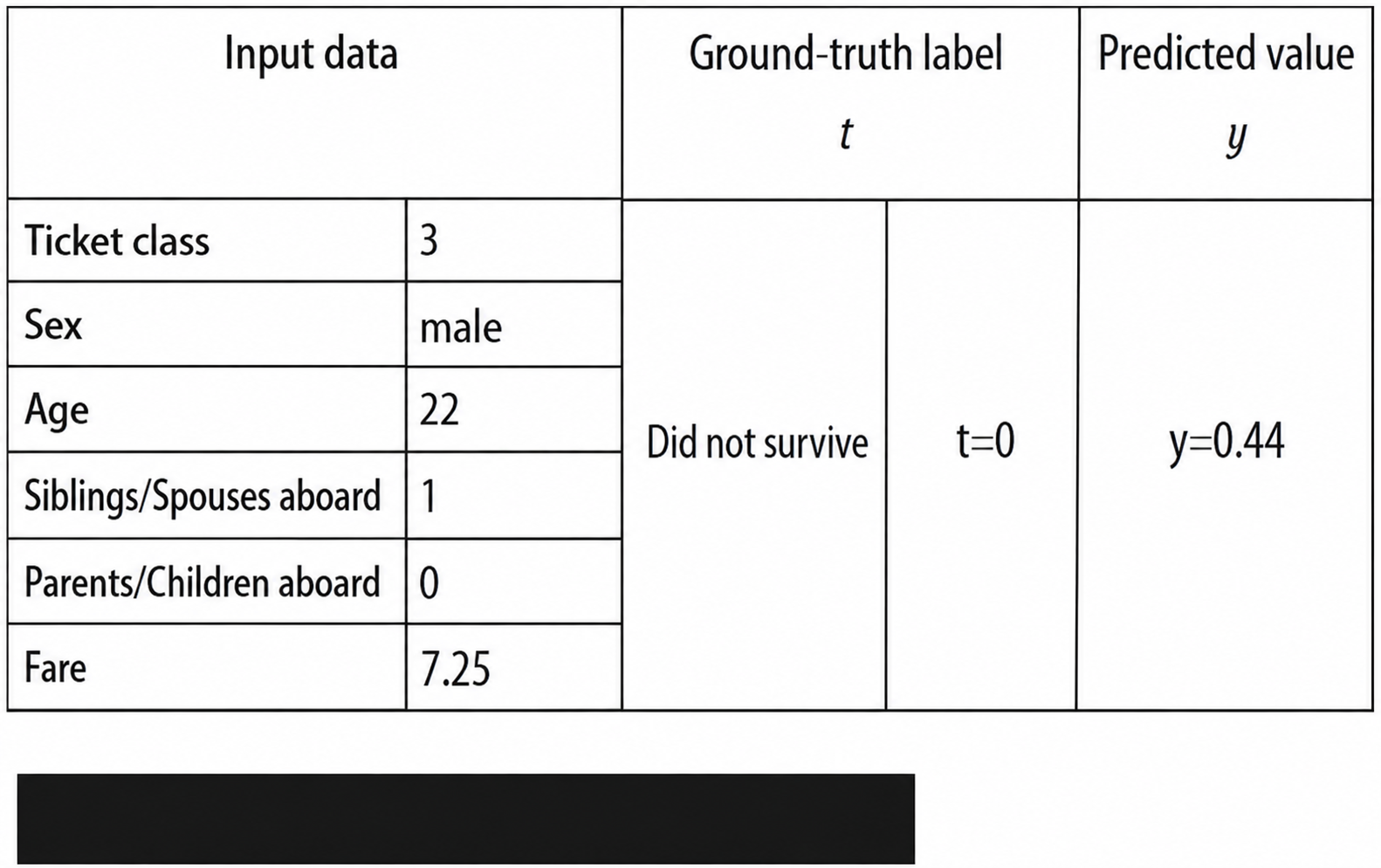
In other words, in multi-class classification there were as many ground-truth labels as classes, \(t_{1}\), \(t_{2}\), and so on, whereas in binary classification we set \(t=1\) when we want the input to be predicted as \(1\), and \(t=0\) when we want the input to be predicted as \(0\).

7-2. Cross-Entropy for Binary Classification (N-Sample Version)

Equation \((7.3)\) was the single-sample cross-entropy function; we now extend it to a binary cross-entropy function that handles N data samples.

$$
BCE=- (t \log y + (1-t) \log (1-y) ) \tag{7.3, restated}
$$

The multiple training samples used in batch learning look like the following. Four samples are shown here.

Each is assigned a data index \(i\). As mentioned earlier, in binary classification there is exactly one ground-truth label and one predicted value per data sample, so attaching the data index \(i\) to the label and predicted value is enough to identify them uniquely.

So we add the data index \(i\) as a subscript to the ground-truth label \(t\), giving \(t_{i}\), and likewise add the data index \(i\) as a subscript to the predicted value \(y\), giving \(y_{i}\).

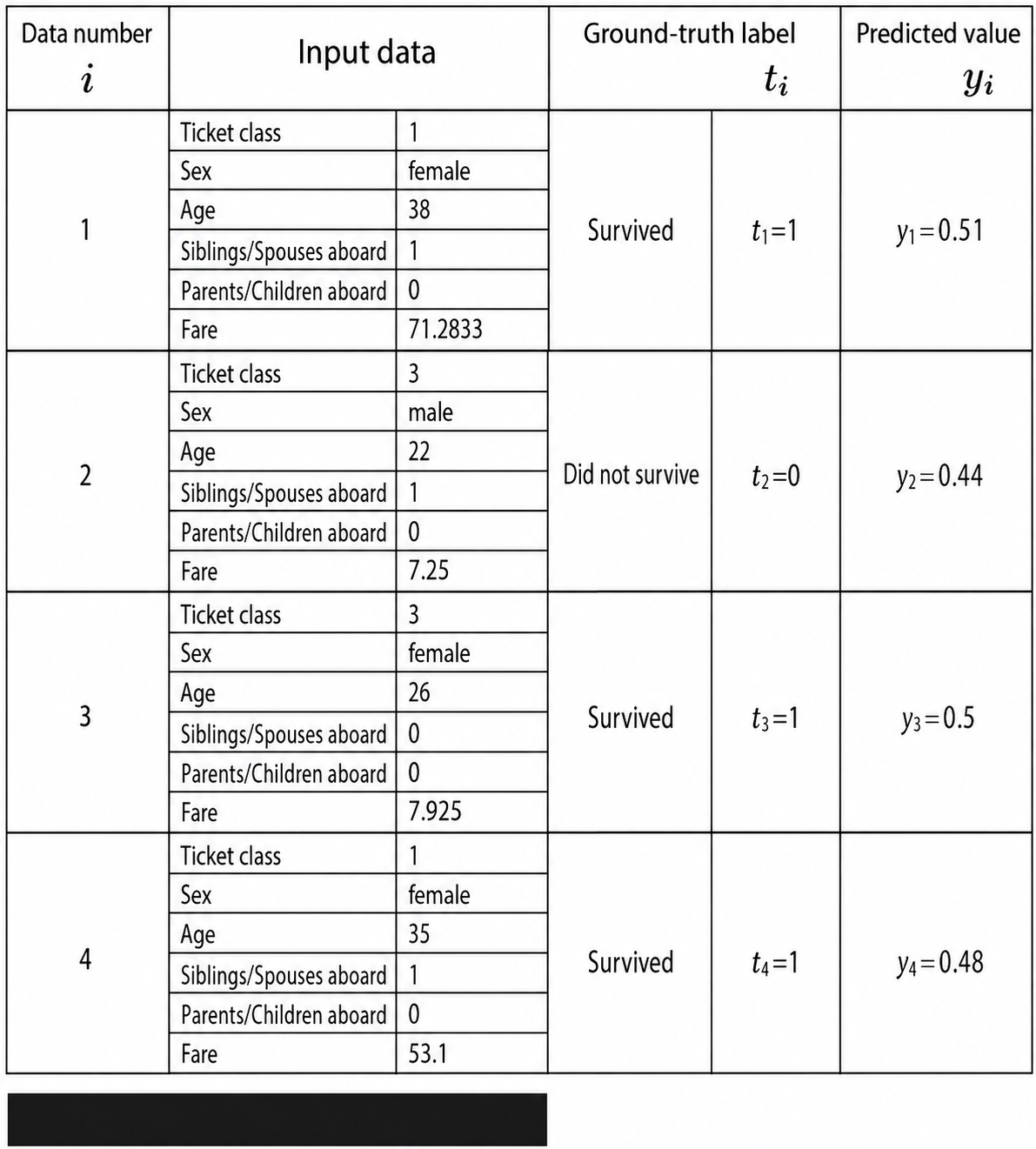
Accordingly, the per-sample binary cross-entropy function, with the data index \(i\) added as a subscript, becomes:

$$
BCE_{i}=- (t_{i} \log y_{i} + (1-t_{i}) \log (1-y_{i}) )
$$

All that remains is to sum this over the N data samples and then divide by N to remove the effect of the number of samples, which yields the batch version of the binary cross-entropy formula, just as in the multi-class case.

$$
\begin{aligned}
BCE=&- \sum_{i=1}^{N} BCE_{i}&\
&- \sum_{i=1}^{N} \lbrack t_{i} \log y_{i} + (1-t_{i}) \log (1-y_{i}) \rbrack &
\end{aligned}
$$

With that, we have derived the cross-entropy for binary classification (batch version).

$$
BCE=- \sum_{i=1}^{N} \lbrack t_{i} \log y_{i} + (1-t_{i}) \log (1-y_{i}) \rbrack \tag{7.4}
$$

$$
t_{i}: \text{ground-truth label of the } i\text{-th sample}\quad y_{i}: \text{predicted value of the } i\text{-th sample}
$$

How was this installment?

See you next time.

References
https://journal.qualiteg.com/books/

navigation