Cross-Entropy Explained, Part 7: Cross-Entropy and Vector Operations

Good morning! This is the Qualiteg Research Team.

In this article, we explain how to express the cross-entropy computation using vectors and matrices.

Chapter 8: Cross-Entropy and Vector Operations

First of all, why would we want to express cross-entropy with vectors and matrices?

The reason is that when you actually implement a neural network as a computer program, training data and predictions are handled as N-th order tensors (N-dimensional arrays) such as vectors (1-dimensional arrays) and matrices (2-dimensional arrays).

As for why vectors and matrices: in practical neural network computation, we do not take out one data item and compute it, then the next, and so on. Instead, we pack many data items into vectors (1-dimensional arrays), matrices (2-dimensional arrays), or even higher-dimensional arrays, and then compute them all in one big batch.

(One could say that deep learning has advanced as far as it has precisely because GPUs, which excel at this kind of bulk computation, exist.)

So, in preparation for implementing on a computer the cross-entropy computation we have derived so far, let's turn it into a 1-dimensional array.

In program code it is just a 1-dimensional array, but we will regard it as a vector whose components are the values of the array.

If we let \(\boldsymbol{t}\) be the vector containing the ground-truth labels \(t_{k}\) as its elements, it becomes a vector with the following components.

$$
\boldsymbol{t} =
\begin{pmatrix}
t_{1} & t_{2} & t_{3}
\end{pmatrix}
$$

In this case, since the components (i.e., the numbers) are laid out horizontally, it is called a row vector (or a horizontal vector).

Similarly, if we express the predictions \(y_{k}\) as a row vector \(\boldsymbol{y}\), we get

$$
\boldsymbol{y} =
\begin{pmatrix}
y_{1} & y_{2} & y_{3}
\end{pmatrix}
$$

Furthermore, when computing cross-entropy, we take the logarithm \(\log\) of the components of \(\boldsymbol{y}\), so if we define \(\boldsymbol{y_{l}}\) as the vector obtained by taking \(\log\) of each component of \(\boldsymbol{y}\), we get the following.

$$
\boldsymbol{y_{l}} =
\begin{pmatrix}
\log y_{1} & \log y_{2} & \log y_{3}
\end{pmatrix}
$$

Now let's recall the cross-entropy \(E\).

$$
\begin{aligned}
\ E = &- \sum_{k=1}^{K} t_{k} \log y_{k} &\
&= - ( t_{1} \log y_{1} + t_{2} \log y_{2} + t_{3} \log y_{3}) & \
\end{aligned}
$$

Take a close look at the \(( t_{1} \log y_{1} + t_{2} \log y_{2} + t_{3} \log y_{3})\) that appears in this expression. You can see that it is the dot product (inner product) of the vector \(\boldsymbol{t}\) and the vector \(\boldsymbol{y_{l}}\).

The dot product (inner product) is the sum of the products of components that share the same index.

$$
\begin{aligned}
\ E =　&- \boldsymbol{t} \cdot \boldsymbol{y_{l}}& \
&= - ( t_{1} \log y_{1} + t_{2} \log y_{2} + t_{3} \log y_{3}) & \
\end{aligned}
$$

One point to be careful about: for vectors, it is enough to define the dot product as the sum of the products of corresponding components, but when computing the dot product of matrices (2-dimensional arrays) rather than vectors, you have to pay attention to the shapes of the matrices.

For example, the dot product of the matrix $\begin{pmatrix}
1 & 2 & 3 \
4 & 5 & 6 \
\end{pmatrix}\( with shape \)2 \times 3\( (rows by columns) and the matrix \)\begin{pmatrix}
7 & 8 \
9 & 10 \
11 & 12 \
\end{pmatrix}$ with shape \(3 \times 2\),

$$
\begin{pmatrix}
1 & 2 & 3 \
4 & 5 & 6 \
\end{pmatrix}
\cdot
\begin{pmatrix}
7 & 8 \
9 & 10 \
11 & 12 \
\end{pmatrix}
$$

is computed as follows.

We add up the products of the components of the first row (running horizontally) of the left matrix and the first column (running vertically) of the right matrix.

Next, we add up the products of the components of the second row of the left matrix and the first column of the right matrix... and continue in the same way from there.

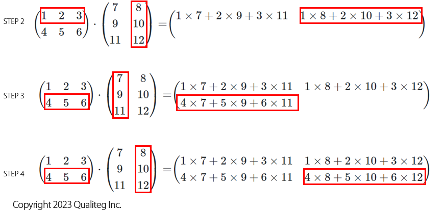
Computing in this order, the result is as follows.

$$
\begin{aligned}
\begin{pmatrix}
1 & 2 & 3 \
4 & 5 & 6 \
\end{pmatrix}
\cdot
\begin{pmatrix}
7 & 8 \
9 & 10 \
11 & 12 \
\end{pmatrix}=&
\begin{pmatrix}
1 \times 7 + 2 \times 9 + 3 \times 11 & 1 \times 8 + 2 \times 10 + 3 \times 12 \
4 \times 7 + 5 \times 9 + 6 \times 11 & 4 \times 8 + 5 \times 10 + 6 \times 12
\end{pmatrix}&\
=&
\begin{pmatrix}
58 & 64 \
139 & 154 \
\end{pmatrix}&
\end{aligned}
$$

As this example shows, the dot product of a matrix with shape \(2 \times 3\) (rows by columns) and a matrix with shape \(3 \times 2\) is a \(2 \times 2\) matrix.

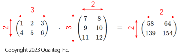
In other words, the dot product of an \(m \times n\) matrix and an \(n \times l\) matrix has shape \(m \times l\).
Also, to compute a dot product, the number of columns of the left matrix must match the number of rows of the right matrix.

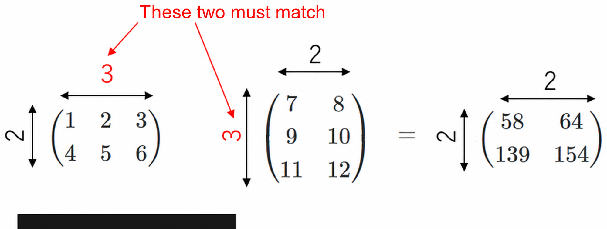
Now that we have seen how to compute the dot product of matrices, let's revisit the dot product of the vectors from earlier.

The row vector \(\boldsymbol{t}\) representing the ground-truth labels and the row vector \(\boldsymbol{y_{l}}\) obtained by taking \(\log\) of the predictions were as follows:

$$
\boldsymbol{t} =
\begin{pmatrix}
t_{1} & t_{2} & t_{3}
\end{pmatrix}
$$

$$
\boldsymbol{y_{l}} =
\begin{pmatrix}
\log y_{1} & \log y_{2} & \log y_{3}
\end{pmatrix}
$$

If we try to compute according to the matrix dot product rule above, we find that we cannot compute the product of two row vectors, both of which are shaped as a single horizontal row.

That is,

$$
\begin{pmatrix}
t_{1} & t_{2} & t_{3}
\end{pmatrix}
\cdot
\begin{pmatrix}
\log y_{1} & \log y_{2} & \log y_{3}
\end{pmatrix}
$$

cannot be computed as it stands.
In other words, if we regard these two row vectors as matrices, both have shape \(1 \times 3\).

Therefore, to get them into the \(m \times n\) and \(n \times l\) shapes that allow a dot product, it looks like we should turn the vector \(\boldsymbol{y_{l}}\) from a row vector (horizontal vector) into a column vector (vertical vector).

The column vector \(\boldsymbol{y_{l}^\mathsf{T} }\), obtained by swapping the rows and columns of the components of \(\boldsymbol{y_{l}}\), looks like this.

(\({\mathsf{T} }\) denotes the transpose. The transpose is the matrix obtained by swapping the rows and columns of the components of a given matrix.)

$$
\boldsymbol{y_{l}^\mathsf{T} } =
\begin{pmatrix}
\log y_{1} \ \log y_{2} \ \log y_{3}
\end{pmatrix}
$$

Now we can compute it following the rules of the dot product.

Looking at the cross-entropy formula using the dot product from earlier,

$$
\begin{aligned}
\ E =　&- \boldsymbol{t} \cdot \boldsymbol{y_{l}^\mathsf{T} }& \
&=-\begin{pmatrix}
t_{1} & t_{2} & t_{3}
\end{pmatrix}
\cdot
\begin{pmatrix}
\log y_{1} \ \log y_{2} \ \log y_{3}
\end{pmatrix}& \
&= - ( t_{1} \log y_{1} + t_{2} \log y_{2} + t_{3} \log y_{3}) & \
\end{aligned}
$$

With this, we have been able to obtain the cross-entropy as a matrix computation.

(Incidentally, since the dot product of two vectors is the same as the inner product, the result of the computation is a scalar, that is, a single number.)

How was this installment?

As mentioned at the beginning, the reason we treated the data as vectors and matrices and computed a dot product is that, in environments that excel at parallel computation such as GPUs, packing the data into vectors and matrices and computing everything at once is overwhelmingly more efficient than looping through the computation one item at a time.

We use this technique precisely because vectors and matrices are a good fit for computers (GPUs in particular) and can be expected to improve computational efficiency and speed. That is what really matters, and there is perhaps no need to read much more mathematical meaning or significance into it beyond that.

See you next time!

References
https://journal.qualiteg.com/books/