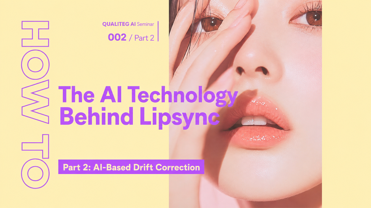
How to Build AI Lipsync, Part 2: AI-Powered Drift Correction
Hello!
In the previous article, we explained the lipsync technology used in our MotionVox service, focusing on how audio features are extracted with wav2vec. You should now have a good grasp of the foundational technology for predicting accurate mouth movements from speech.
This time, as a sequel, we focus on cumulative drift — a key technical challenge in lipsync production. Even with highly accurate phoneme recognition from wav2vec, when multiple audio segments are arranged along a timeline in actual video production, tiny timing errors accumulate and eventually become a noticeable offset.
In this article, we take a detailed look at the mechanism of cumulative drift and at modern, machine-learning-based correction techniques, illustrated with real measurement data. Combining the wav2vec feature extraction from last time with the drift-correction techniques covered here should give you the full picture of how MotionVox achieves high-quality lipsync.
What Is Cumulative Drift?
Basic Concept
Cumulative drift is the phenomenon in which the tiny timing errors of individual audio segments build up over time.
Segment 1: +0.5 ms error
Segment 2: -0.3 ms error
Segment 3: +0.8 ms error
...
After 100 segments: 42 ms of total drift
A Real Measurement Example
Below is actual cumulative-drift measurement data for roughly seven minutes of audio content
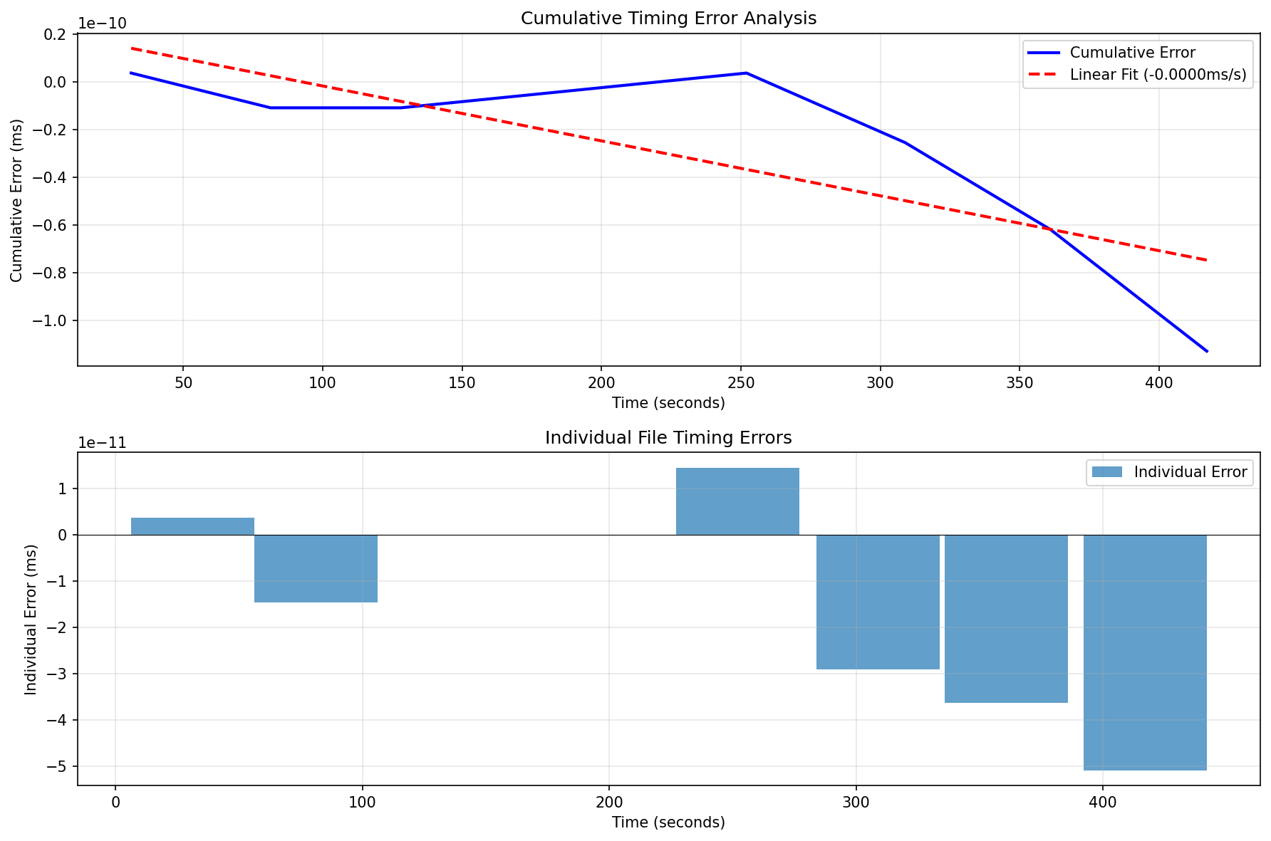
Top graph: cumulative timing error
- Solid blue line: the actual cumulative error over time
- Dashed red line: linear fit (-0.0000 ms/s)
- The vertical scale is extremely small, on the order of 10^-10 — technically near-perfect accuracy
Bottom graph: timing error of individual files
- The error of each audio file is on the order of 10^-11 milliseconds
- Positive and negative errors are mixed, so a canceling effect is at work
These measurements reveal an interesting fact:even though synchronization is technically accurate to near the limits of measurement, viewers can still sometimes sense a subtle offset — a curious phenomenon.
Why Does Lipsync Go Out of Sync?
1. The Discrete Nature of Digital Audio
Digital audio's time resolution is determined by its sampling frequency
# For 48 kHz sampling
time_resolution = 1 / 48000  # about 0.021 ms

# To represent 1.5 seconds
ideal_samples = 1.5 * 48000  # 72,000 samples
actual_duration = 72000 / 48000  # exactly 1.5 seconds
2. File-Format Constraints
Mismatches between an audio file's header information and its actual sample count
- Rounding errors in metadata
- Differences between encoder implementations
- Errors introduced during format conversion
3. Precision of Processing Tools
Differences in processing precision across audio-editing software and libraries
- Truncation and rounding at frame boundaries
- Accumulated floating-point arithmetic errors
- Interpolation errors during resampling
The Gap Between Human Perception and Technical Accuracy
Perceptual Thresholds
The human auditory and visual systems have the following characteristics:
| Delay | Perceptual impact |
|---|---|
| 0-20 ms | Virtually imperceptible |
| 20-40 ms | Sensitive viewers notice something is off |
| 40-80 ms | Most people notice something is off |
| 80 ms and above | The offset is clearly perceived |
As the measurement data above shows, perceptual discomfort can arise even when the technical error is essentially zero. Possible reasons include
- Video-processing latency
- Playback-device delay
- Psychoacoustic factors
and the like.
Drift Analysis Methods
Now let's look at how drift is actually analyzed
1. Measuring the Error
First, measure the difference between the expected and actual duration of each audio segment
def measure_segment_error(expected_duration, actual_duration):
    """Measure the error of each segment"""
    error_ms = (actual_duration - expected_duration) * 1000
    return {
        'absolute_error': abs(error_ms),
        'signed_error': error_ms,
        'relative_error': error_ms / (expected_duration * 1000)
    }
2. Analyzing the Accumulation Pattern
Next, model how the errors accumulate
def analyze_accumulation_pattern(errors, timestamps):
    """Analyze the accumulation pattern"""
    cumulative = np.cumsum(errors)

    # Linear model: drift = a * time + b
    linear_fit = np.polyfit(timestamps, cumulative, 1)

    # Quadratic model: drift = a * time² + b * time + c
    quadratic_fit = np.polyfit(timestamps, cumulative, 2)

    # Evaluate model goodness of fit
    linear_r2 = calculate_r_squared(cumulative, linear_fit)
    quadratic_r2 = calculate_r_squared(cumulative, quadratic_fit)

    return {
        'pattern': 'linear' if linear_r2 > 0.9 else 'nonlinear',
        'drift_rate': linear_fit[0],  # ms/second
        'acceleration': quadratic_fit[0] if quadratic_r2 > linear_r2 else 0
    }
3. Understanding the Statistical Characteristics
Finally, characterize the errors statistically
def statistical_analysis(errors):
    """Analyze the statistical characteristics of the errors"""
    return {
        'mean': np.mean(errors),
        'std': np.std(errors),
        'skewness': scipy.stats.skew(errors),
        'is_systematic': abs(np.mean(errors)) > np.std(errors) / 2
    }
So far we have looked at methods for analyzing the drift.
Now let's take a quick look at how to correct it, starting with the classic techniques
Traditional Correction Methods
Once drift analysis has revealed the pattern of cumulative error, the next step is correction. Before bringing in machine learning, let's first review the basic correction methods that have long been in use. They are computationally light and simple to implement, and they still work well in many situations.
1. Static Offset Correction
Apply a constant correction across the board
def static_offset_correction(position, offset_ms, sample_rate):
    """Correction with a fixed offset"""
    offset_samples = int(offset_ms * sample_rate / 1000)
    return position + offset_samples
When to use
- When there is a systematic delay or lead
- When the drift rate is very small
2. Linear Correction
Apply a correction proportional to time
def linear_correction(position, time, drift_rate, sample_rate):
    """Linear drift correction"""
    # drift_rate: ms/second
    correction_ms = -drift_rate * time
    correction_samples = int(correction_ms * sample_rate / 1000)
    return position + correction_samples
When to use
- When drift progresses at a constant rate
- For cumulative error in long-form content
3. Adaptive Correction
Compute the optimal correction for each segment
def adaptive_correction(segments, measured_errors):
    """Adaptive correction algorithm"""
    corrections = []
    accumulated_error = 0

    for i, segment in enumerate(segments):
        # Cumulative error so far
        accumulated_error += measured_errors[i]

        # Predict future errors
        future_segments = len(segments) - i - 1
        predicted_future_error = np.mean(measured_errors) * future_segments

        # Compute the optimal correction
        optimal_correction = -(accumulated_error + predicted_future_error * 0.5)
        corrections.append(optimal_correction)

    return corrections
4. Smooth Correction via Spline Interpolation
from scipy.interpolate import UnivariateSpline

def spline_correction(timestamps, cumulative_errors, smoothing_factor=0.1):
    """Smooth correction via spline interpolation"""
    # Generate the correction curve
    spline = UnivariateSpline(timestamps, -cumulative_errors,
                              s=smoothing_factor)

    # Compute the correction at each time point
    corrections = spline(timestamps)
    return corrections
The Limits of Traditional Methods — and What Machine Learning Promises
The traditional correction methods we have seen are effective in many cases. In particular, when the drift pattern is simple and predictable, these methods alone can deliver high-quality lipsync.
In real production settings, however, we sometimes face more complicated situations
- Nonlinear, complex drift patterns➡ Complex error accumulation that simple formulas cannot express
- Content-dependent variation➡ Drift that changes with speaker characteristics, speaking rate, emotional expression, and more
- Unpredictable disturbances➡ Unexpected delays introduced by encoding, editing, or the playback environment
For these challenges, traditional methods hit their limits. This is where next-generation, machine-learning-based drift correction comes in. With the flexibility to learn complex patterns from large amounts of data and adapt to unseen situations, machine learning promises a further leap in lipsync quality.
Advanced Correction with Machine Learning
For complex drift patterns that traditional correction methods struggle with, machine learning offers an innovative approach.
Let's look at how the power of AI enables more sophisticated drift correction.
Machine learning's greatest strength is its ability to learn complex patterns automatically from data, without explicit programming. For lipsync drift correction, it can learn from a large body of past project data which kinds of drift occur under which conditions, and then predict appropriate corrections for new content.
1. Time-Series Prediction with LSTMs
Learn cumulative drift patterns and predict future errors
import tensorflow as tf

class DriftPredictionLSTM:
    def __init__(self, sequence_length=10):
        self.model = tf.keras.Sequential([
            tf.keras.layers.LSTM(64, return_sequences=True),
            tf.keras.layers.LSTM(32),
            tf.keras.layers.Dense(16, activation='relu'),
            tf.keras.layers.Dense(1)
        ])

    def train(self, historical_errors, timestamps):
        """Learn drift patterns from past projects"""
        X, y = self.create_sequences(historical_errors)
        self.model.compile(optimizer='adam', loss='mse')
        self.model.fit(X, y, epochs=100, validation_split=0.2)

    def predict_drift(self, recent_errors):
        """Predict the drift of the next segment"""
        return self.model.predict(recent_errors.reshape(1, -1, 1))
2. Adaptive Correction with Reinforcement Learning
Optimize the correction strategy based on feedback from the environment
class AdaptiveCorrectionRL:
    def __init__(self, state_dim=5, action_dim=11):
        # State: [cumulative error, current position, error variance, remaining segments, last correction]
        # Actions: corrections from -5 ms to +5 ms (in 1 ms steps)
        self.q_network = self.build_q_network(state_dim, action_dim)
        self.memory = []

    def build_q_network(self, state_dim, action_dim):
        model = tf.keras.Sequential([
            tf.keras.layers.Dense(64, activation='relu', input_shape=(state_dim,)),
            tf.keras.layers.Dense(32, activation='relu'),
            tf.keras.layers.Dense(action_dim)
        ])
        return model

    def choose_action(self, state, epsilon=0.1):
        """Choose the correction amount with an ε-greedy policy"""
        if np.random.random() < epsilon:
            return np.random.randint(-5, 6)  # Exploration
        else:
            q_values = self.q_network.predict(state.reshape(1, -1))
            return np.argmax(q_values) - 5  # Exploitation

    def update(self, state, action, reward, next_state):
        """Update the Q-values"""
        # Deep Q-Learning update step
        pass
3. Pattern Recognition with Convolutional Neural Networks
Detect drift patterns directly from the audio waveform
class WaveformDriftDetector:
    def __init__(self):
        self.model = tf.keras.Sequential([
            # Extract waveform features with 1D convolutions
            tf.keras.layers.Conv1D(32, 128, activation='relu'),
            tf.keras.layers.MaxPooling1D(4),
            tf.keras.layers.Conv1D(64, 64, activation='relu'),
            tf.keras.layers.GlobalMaxPooling1D(),

            # Predict the error with fully connected layers
            tf.keras.layers.Dense(128, activation='relu'),
            tf.keras.layers.Dropout(0.5),
            tf.keras.layers.Dense(1)  # Predicted error (ms)
        ])

    def detect_inherent_delay(self, waveform):
        """Detect inherent delay from the waveform"""
        # Estimate encoding-induced delay from
        # characteristics such as the audio onset
        features = self.extract_features(waveform)
        return self.model.predict(features)
4. Robust Correction with Ensemble Learning
Combine multiple methods to improve reliability
class EnsembleDriftCorrector:
    def __init__(self):
        self.correctors = [
            LinearCorrector(),
            SplineCorrector(),
            LSTMPredictor(),
            RLCorrector()
        ]
        self.weights = [0.25, 0.25, 0.25, 0.25]

    def correct(self, segment_info):
        """Weighted average of multiple correction methods"""
        corrections = []
        for corrector, weight in zip(self.correctors, self.weights):
            correction = corrector.predict(segment_info)
            corrections.append(correction * weight)

        # Average with outliers excluded
        final_correction = np.median(corrections)
        return final_correction

    def adapt_weights(self, performance_metrics):
        """Adjust weights based on each method's performance"""
        # Learn optimal weights via meta-learning
        pass
The Practical Value of Machine Learning Methods
Machine-learning-based correction delivers value that traditional methods could not
1. Handling complexity
- Can learn nonlinear, hard-to-predict drift patterns
- Handles compound errors driven by multiple interacting factors
2. Adaptability and generalization
- Adapts flexibly to new types of content and new speakers
- A system that keeps improving as training data grows
3. Automation and efficiency
- No manual parameter tuning required
- Fast, real-time processing is achievable
4. Continuous improvement
- Self-improvement through feedback loops
- Always reflects the latest data trends
These machine learning methods are powerful on their own, but combining them with traditional methods yields an even more robust and practical system. For example, a hybrid approach is effective: use basic linear correction for the coarse adjustment, then let machine learning correct the complex error patterns that remain.
In the next section, we look at the implementation considerations for integrating these techniques into a real workflow.
A Practical Workflow
We have covered both traditional methods and machine-learning-based correction — but how are these techniques actually combined in production? Here we describe a workflow for putting the theory into practice.
Effective drift correction does not rely on a single technique; the key is selecting and combining the right methods for each situation. Below is a step-by-step approach based on our hands-on experience with MotionVox.
- Initial analysis
- Measure the error of every segment
- Identify the accumulation pattern
- Prepare training data for the machine learning models
- Choosing a correction strategy
- Linear drift → linear correction + LSTM prediction
- Random errors → adaptive correction + reinforcement learning
- Complex patterns → ensemble methods
- Parameter tuning
- Hyperparameters of the machine learning models
- Correction strength and smoothing
- Validation and feedback
- Perceptual evaluation via A/B testing
- Continuous model improvement
Toward Further Improvement
The current workflow is already quite practical, but further evolution lies ahead. We envision a real-time diagnostic system that instantly classifies the type of problem and automatically selects the best correction method, and mechanisms that incorporate models of human audiovisual perception to close the gap between technical accuracy and perceived quality. Lightweight models could enable real-time processing on edge devices, and explainability features — letting the AI explain why it chose a particular correction — would enable better collaboration between creators and AI. Through these improvements, we aim for a lipsync system that is more intuitive, faster, and more reliable.
Summary
Lipsync quality is a crucial factor in how immersed viewers feel. As we have seen in this article, audio synchronization is now technically possible with extremely high precision, yet fully satisfying human perception requires further ingenuity.
By introducing machine learning, we can now address challenges that deterministic approaches struggled with
- Predicting and correcting nonlinear drift patterns
- Adaptive adjustment based on content characteristics
- Improving accuracy by learning from past projects
- Fast decision-making for real-time processing
Going forward, demand for even more advanced lipsync will grow — not only for pre-generated photorealistic avatars but also for real-time avatar control in metaverse spaces. Through advances in machine learning models, a deeper understanding of human perception, and our relentless pursuit of realism, we aim to achieve completely natural lipsync!
See you next time!