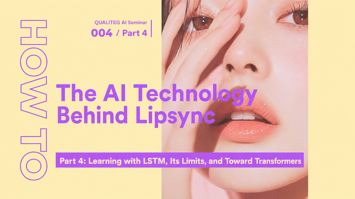
How to Build AI Lipsync, Part 4: Training LSTMs, Their Limits, and the Leap to Transformers

Hello! Welcome to Part 4 of our lip-sync technology series!
In the previous installment (Part 3), we began exploring the core technology of converting wav2vec features into mouth-shape parameters. We looked at the complex relationship between speech and mouth shapes—especially coarticulation, where the same phoneme changes with context—and then covered the LSTM approach to this time-series problem, from the long-term memory enabled by LSTM gate mechanisms all the way to actual network design.
This time, we explain in detail how to actually train that LSTM, from data preparation through the training process.
Then, after laying out the limits of LSTMs, we introduce the Transformer, a newer approach that overcomes them.
1. Data Preparation: Balancing Quality and Quantity
1.1 The Types of Data You Need (Audio, Mouth Shapes, Synchronization)
Training a high-quality lip-sync model requires three kinds of data. Each comes with strict quality requirements, and if they are not met, even the best network architecture will not produce good results.
First, the audio data: a sampling rate of 16kHz or higher is mandatory. This is because wav2vec is trained at 16kHz; lower sampling rates lose phonetic information. The recording environment also matters—recording in a soundproof room with little background noise is ideal. As for speakers, professional voice actors or announcers with clear articulation are preferable, but ordinary speakers work too if they enunciate carefully.
Next, the mouth-shape data. There are various approaches here. Sometimes we use image-analysis pipelines that can track facial landmarks in 3D; in other cases, to capture facial landmarks from scratch, we attach fluorescent markers to the face and track them three-dimensionally with multiple cameras to record precise mouth movements.
As for the capture equipment, the frame rate ideally needs to be 60fps or higher.
Human mouth movements are surprisingly fast—plosives in particular involve large changes within 20 milliseconds—which is why a high frame rate is necessary.
For 4K capture at 60 or 120 FPS, you will want a high-end digital camera or camcorder, such as an α7 IV or an FX3. Data is everything here, so do not skimp on preparation or equipment.
And the most important element of all is synchronization between audio and mouth shapes. Even a 50-millisecond offset registers as unnatural to the human eye. During recording, therefore, you need a timecode-based system that keeps audio and video perfectly in sync.
1.2 Techniques for Training an LSTM with Minimal Data
In machine learning, the conventional wisdom is "the more data, the better," but collecting high-quality motion-capture data costs enormous time and money. So you need techniques for learning effectively even from limited data.
Another technique for efficient training is designing the dataset around phoneme balance. In Japanese, "あ" (a) and "い" (i) appear frequently, while "ぢ" (di) and "づ" (du) are rare. Instead of recording every phoneme equally, adjusting the number of recordings to match real-world frequency lets you build an efficient dataset.
1.3 Efficient Training Through Data Augmentation
To extract the maximum learning effect from limited data, we use a technique called data augmentation: applying various transformations to existing data to effectively increase its volume.
For audio data, changing the speaking rate is effective. Stretching or compressing the original audio between 0.8x and 1.2x lets the model learn a range of speaking rates, from slow speech to rapid speech. Note that the mouth-shape data must be stretched by the same ratio.
Adding slight noise also helps. Real-world environments are never perfectly silent, so adding moderate noise produces a more robust model. If the noise is too strong, however, phonetic information is damaged, so the signal-to-noise ratio should be kept at 20dB or higher.
Small shifts along the time axis are another effective augmentation technique. Randomly offsetting the audio/mouth-shape synchronization within ±30 milliseconds trains a robust model that works even when synchronization is imperfect. This builds tolerance to the sync drift that can occur in real applications.
Combining these augmentation techniques can generate 10 to 20 times the original volume of effective training data. Turning 1,000 original samples into 10,000 to 20,000 training samples makes it possible to train a high-quality model even on a limited recording budget.
2. The LSTM Training Process: Why It Can Learn from Little Data
2.1 The Strength of a Time-Series Inductive Bias
One reason LSTMs can learn effectively from small datasets is that they carry an "inductive bias."An inductive bias is the "preferred direction of learning" built into a model; in the case of LSTMs, the assumption that "time-series data should be processed in order" comes built in.
This inductive bias resembles how humans learn. When we learn language, we instinctively understand that the order of sounds matters. Nobody has to teach us that "こんにちは" (konnichiwa, "hello") and "はちにんこ" (hachininko—the same syllables reversed) mean completely different things—it is too obvious to even mention. Likewise, an LSTM "knows" that temporal order matters, which is why it can learn patterns efficiently from little data.
2.2 A Staged Training Strategy (Vowels → Consonants → Complex Phonemes)
Another key to efficient training is a staged strategy. Rather than throwing complex sentences at the model from the start, we begin with easy material and gradually raise the difficulty.
In stage one, the model learns only the five Japanese vowels (あ・い・う・え・お). Vowel mouth shapes are relatively simple and change smoothly, making them easy targets for an LSTM. This stage establishes the basic open/close patterns of the mouth and their correspondence with the audio features. A few hundred samples are usually enough to learn most of the basic vowel patterns.
In stage two, we add plosives (the p-, b-, and t-rows of the kana table, and so on) and fricatives (the s- and h-rows, etc.). These consonants produce distinctive changes in mouth shape and therefore require learning different patterns from vowels. But because the correspondence for the basic patterns was learned in stage one, the new patterns are picked up fairly efficiently.
In stage three, the model learns natural sentences containing all phonemes. At this stage it learns more complex phenomena, such as coarticulation and long-range dependencies. The knowledge acquired in earlier stages serves as the foundation on which more advanced patterns are built up.
2.3 Loss Function Design for Efficient Training
Another important factor in boosting training efficiency is designing an appropriate loss function.Rather than simply minimizing the difference between predicted and ground-truth values, we perform optimization from multiple perspectives directly tied to lip-sync quality.
First is a loss for positional accuracy. For each of the 26 mouth-shape parameters, we compute the difference between the predicted and ground-truth values. However, instead of weighting every parameter equally, visually important parameters (jaw_open, mouth_open, and the like) are given larger weights. This concentrates the limited learning capacity on the parts that matter most.
Next is a loss for temporal smoothness. Physical constraints prevent the human mouth from changing drastically in an instant. So we also include the amount of change between consecutive frames in the loss function. This prevents choppy, unnatural movement and teaches the model smooth mouth motion.
We further add constraints on velocity and acceleration. There are limits to how fast a mouth can open and close, and abrupt acceleration or deceleration looks unnatural. Building these physical constraints into the loss function teaches more human-like movement.
An Example Loss Function
L_total = λ₁L_position + λ₂L_velocity + λ₃L_acceleration + λ₄L_smoothness + λ₅L_phonemeNow let's look at each term in detail.
Computes the difference between predicted and ground-truth values at each time step. Important parameters (jaw opening, mouth opening) receive larger weights.
Computes the change between consecutive frames (first derivative). Constrains the mouth from opening or closing too abruptly.
Computes the rate of change of velocity (second derivative). Suppresses abrupt acceleration and deceleration for physically natural movement.
Minimizes the rate of change of acceleration (third derivative = jerk). Natural human movement is smooth, with no abrupt changes.
Estimates the phoneme back from the predicted mouth shape and checks whether it matches the original phoneme. A bidirectional consistency check.
These weights are adjustable and tuned per use case. For example, you might emphasize smoothness for an animated character, or positional accuracy for a photorealistic human—optimizing for whatever the goal is.
velocity = (current position - position 1 second ago) ÷ 1 second
acceleration = (current velocity - velocity 1 second ago) ÷ 1 second
jerk = (current acceleration - acceleration 1 second ago) ÷ 1 second
• Position only → teleporting allowed (bad)
• Position + velocity → sudden starts and stops allowed (still bad)
• Position + velocity + acceleration → jittery movement allowed (almost there)
• All of them → natural, smooth movement (perfect!)
      Frame 1: mouth opening = 0mm

      Frame 2: mouth opening = 5mm

      Frame 3: mouth opening = 12mm

      Frame 4: mouth opening = 18mm
      Velocity at frame 2 = (5mm - 0mm) ÷ (1/60 s) = 300mm/s

      Velocity at frame 3 = (12mm - 5mm) ÷ (1/60 s) = 420mm/s

      Velocity at frame 4 = (18mm - 12mm) ÷ (1/60 s) = 360mm/s
      Acceleration at frame 3 = (420 - 300) ÷ (1/60 s) = 7200mm/s²

      Acceleration at frame 4 = (360 - 420) ÷ (1/60 s) = -3600mm/s²
1. Filming stays simple - you only need to capture positions
2. Noise resistance - you can apply filtering when differentiating
3. Leveraging physics - you can add constraints like "acceleration this abrupt is impossible"
      Ground truth: position → compute velocity → compute acceleration

      Prediction: position → compute velocity → compute acceleration

             ↓

         Compare at each level and apply penalties
Phonetic-consistency loss also matters. We estimate the phoneme back from the predicted mouth shape and check whether it matches the original phoneme. This verifies that the correspondence between sound and mouth shape has been learned correctly. This bidirectional consistency check makes the training more reliable.
By combining these loss functions appropriately, an LSTM can capture the essence of the human speech mechanism even from little data. With each loss term guiding the training from a different angle, learning becomes both efficient and effective.
3. The Limits of LSTMs: The Problem of Not Seeing Far Away
3.1 Information Decay from Sequential Processing
LSTMs are excellent time-series models, but they carry a fundamental limitation. Their biggest problem is "information decay," which stems from their sequential processing structure.
At each time step, an LSTM receives information from the previous step, processes it, and passes it on to the next. Along the way, the information is inevitably transformed, and some of it is lost. The gate mechanism preserves information longer than a plain RNN can, but there are still limits. In particular, experiments confirm that information from more than 20 steps away fades considerably.
3.2 The Problem with Long Sentences: Information 20 Steps Away Fades
In real lip-sync tasks, this problem has a serious impact. For example, consider the sentence "私は昨日、友達と一緒に映画を見に行って、とても感動しました" ("Yesterday I went to see a movie with a friend, and it really moved me").
This sentence consists of roughly 20 phonemes. By the time the model predicts the mouth shape for the sentence-final "ました" (mashita), almost none of the information from the sentence-initial "私は" (watashi wa) remains. Yet in actual speech, there are features that stay consistent from start to finish—the intonation pattern of the whole sentence, the speaker's emotional state, and so on. LSTMs cannot adequately capture these long-range dependencies.
Japanese honorific expressions make things even trickier. "行きます" (ikimasu, "I will go") and "行きました" (ikimashita, "I went") differ only in their final syllables, yet the articulation pattern of the whole sentence actually differs subtly between them. Polite speech tends to involve clearer mouth movements overall, but by the time an LSTM reaches the end of the sentence, this stylistic information has already been lost.
3.3 Problems Even Bidirectionality Cannot Fully Solve
As introduced in the previous article, a bidirectional LSTM can also use future information, which alleviates the problem to some extent. But it is still not a fundamental solution.
Even in a bidirectional LSTM, information decays in both the forward and backward directions. For instance, when processing the middle (15th) phoneme of a 30-phoneme sentence, the forward LSTM has already lost much of the first five phonemes or so, while the backward LSTM has lost much of the last five. In other words, information from both ends of the sentence cannot be fully utilized.
Bidirectional LSTMs also have a structural constraint. The forward and backward information is eventually combined, but that combination is nothing more than simple concatenation or addition. Complex operations such as "directly comparing information at the start of the sentence with information at the end" are not something it handles well. These limits become problematic in situations such as: long exclamatory sentences where the emotion at the start influences the mouth movement of the whole sentence; questions where the sentence-final interrogative determines the intonation of the entire sentence; and sentences with complex subordinate clauses where the relationship between the main and subordinate clauses must be understood correctly.
To solve this long-range dependency problem at its root, we need a mechanism that can reference information from every position simultaneously and directly, rather than processing it sequentially.
Enter the Transformer—the approach that solves exactly this problem!
4. The Transformer Revolution: Seeing Everything at Once
4.1 The Basic Concept of Self-Attention
The heart of the Transformer is an innovative mechanism called Self-Attention. Where an LSTM processes information in order, Self-Attention can reference the information at every position simultaneously and directly.
To understand the difference, first consider how humans read. When we read a sentence, we do not necessarily process it one character at a time in order. Our eyes jump to important words, moving back and forth between related parts as we grasp the overall meaning. Self-Attention is a mechanism that mimics exactly this human cognitive process.
Self-Attention proceeds in three steps. First, from the information at each position, it generates three vectors: a Query, a Key, and a Value. Next, it computes the similarity between Queries and Keys across all positions to decide where to attend. Finally, it takes a weighted sum of the Values according to those attention scores, producing a new representation for each position.
4.2 Why It Can "See Far": The Power of Parallel Processing
The reason Self-Attention can "see distant information" lies in its parallel processing. In an LSTM, information propagates sequentially, so distant information inevitably decays; Self-Attention instead computes the relationship between every pair of positions directly.
Suppose we have a 50-phoneme sentence. In an LSTM, information from the 1st phoneme needs 49 hops to reach the 50th. If each step multiplies the information by 0.95, it ends up decayed to 0.95^49 ≈ 0.08 of its original strength.
Self-Attention, by contrast, computes the relationship between the 1st and 50th phonemes directly. No matter what lies in between, if these two positions are strongly related, they can form a strong connection. There is no information decay at all.
4.3 Concrete Benefits for Lip-Sync
Self-Attention brings the following benefits to lip-sync tasks in particular.
First, stylistic consistency can be maintained across long sentences. For example, in the sentence
"私は昨日、友達と一緒に映画を見に行って、とても感動しました"
, the speaker information in the sentence-initial "私は" (watashi wa, "I") and the emotional expression in the sentence-final "感動しました" (kandou shimashita, "was deeply moved") can be linked directly. This makes it possible to maintain a consistent style of mouth movement across the entire sentence.
Second, complex coarticulation patterns become learnable. In Japanese, the mouth shape for "っ" (the geminate consonant) depends heavily on the consonants around it, but Self-Attention can assign appropriate attention to the neighboring phonemes and predict the correct mouth shape.
Prosody-pattern capture also improves. In a question, the rising intonation at the end affects the entire sentence; Self-Attention can directly relate the sentence-final interrogative to every position in the sentence, learning the appropriate prosodic pattern.
Self-Attention also offers a major benefit in interpretability. Because you can visualize which phonemes attend to which, you can understand why the model predicted a given mouth shape—extremely useful for improving and debugging the model. In this way, the Transformer's Self-Attention mechanism fundamentally solves the LSTM's long-range dependency problem and enables higher-quality lip-sync generation.
Summary and a Look Ahead
This installment started with the LSTM training process, laid out its limitations, and then introduced the Transformer as an innovative alternative.
In data preparation, we learned techniques for effective training with limited resources. Through data augmentation to multiply effective data volume, a staged training strategy for efficient knowledge acquisition, and loss-function design that optimizes from multiple perspectives, we saw that an LSTM can reach practical performance even with little data.
But we also saw that LSTMs carry a fundamental limitation: information decay caused by sequential processing. The Transformer solves this with its Self-Attention mechanism, which references the information at every position simultaneously and directly—fundamentally resolving the long-range dependency problem and producing more natural, more consistent lip-sync.
In the next installment (Part 5), we will dig into concrete Transformer network designs and the practical challenges of implementing them. We will also introduce hybrid approaches that combine the strengths of LSTMs and Transformers, offering guidance for real-world technology choices—which technique to pick in which situation, drawing on our experience in actual product development. Stay tuned!