The Reality of LLM Training: From GPU Selection to Training Costs

Hello!
Why can OpenAI and Anthropic build world-class LLMs while no LLM from Japan stands shoulder to shoulder with them?
Is it a gap in technical capability? A talent problem?
The answer is simpler than that: the number of GPUs, and money.
Today we focus on "LLM training" and take an in-depth look at the reality behind it.
1. Introduction
"I'd like to try training an LLM myself."
The moment you have that thought, the first wall you hit is the GPU question.
Which GPU, and how many? Should you rent in the cloud or buy on-premises? Is LLM training even realistic for an individual or a small team in the first place?
In this article, we answer these questions with concrete numbers and real-world examples.
For instance, training LLaMA 2 used 2,048 A100s. DeepSeek-V3 cost roughly 800 million yen. So what can you accomplish with the GPUs you actually have? That is what we aim to clarify.
The intended audience is engineers and researchers interested in LLM training. We assume you have written models in PyTorch, but we have tried to keep the article readable even without distributed training experience.
2. Choosing Between GPU Cloud and On-Premises
The Reality of Cloud GPUs
A look at GPU cloud services shows that a wide range of GPUs can be rented by the hour. On "GPU cloud" services, an A6000 starts at a few tens of yen per hour, and an A100 80GB at a few hundred yen. At first glance this looks convenient—but should you rent cloud GPUs, or procure your own GPUs and build a machine on-premises?
Let's run the numbers from a cost perspective. Renting an A100 80GB in the cloud costs at least around 300 yen per hour even on cheaper services. At 8 hours a day, 20 days a month, that is about 48,000 yen per month—roughly 600,000 yen per year. Meanwhile, a used A100 80GB goes for around 1.8 million yen, so it pays for itself in about three years. (That said, they rarely appear on the used market in the first place—which is the frustrating part.)
| Item | Cloud (3 years) | On-premises (3 years) |
|---|---|---|
| Upfront cost | ¥0 | ≈¥1.8M |
| Monthly cost | ≈¥48K | ≈¥10K (electricity) |
| 3-year total | ≈¥1.73M | ≈¥2.16M |
| Usage hours | 160 hours/month | Unlimited |
At around 8 hours of use per day the two are roughly even, but the more hours you use, the more on-premises wins. For workloads that run training around the clock, on-premises is overwhelmingly cheaper.
On-premises does come with hidden costs, though: electricity, cooling, and physical space. An A100 draws 400W and an H100 draws 700W. Run eight H100s around the clock and the electricity bill alone reaches tens of thousands of yen per month.
Even so, if your LLM training fits within a few GPUs, on-premises is well worth considering.
But can you really get by with just a few? Later in this article, we will see just how many GPUs serious full-scratch LLM training actually requires.
Where GPUs Are Actually Used: Training or Inference?
Let's think about global GPU demand for a moment.
What are people using GPUs for LLM work actually doing?
The answer: mostly inference.
When you call an API for a service like ChatGPT, GPUs behind the scenes are running inference. Running RAG (Retrieval-Augmented Generation), generating images—it is all inference.
| Use | Share (est.) | Examples |
|---|---|---|
| Inference | 90%+ | API serving, RAG, chatbots |
| Fine-tuning | A few % | LoRA, QLoRA |
| Full-scratch training | Under 1% | OpenAI, Google, Meta, etc. |
Only a handful of companies—OpenAI, Google, Meta, Anthropic—perform full-scratch training of high-performance LLMs.
In other words, when people talk about "GPUs for LLMs," for most of them it is a conversation about inference GPUs; full-scratch training is an extremely specialized workload.
3. Distributed Training Basics
Why Distributed Training Is Necessary
Now let's return to LLM training.
A single GPU is nowhere near enough for LLM training, for two reasons.
The first is VRAM (GPU memory). How much VRAM does it take to train a 7-billion-parameter (7B) model in FP16?
| Item | Required VRAM |
|---|---|
| Model weights (FP16) | 14GB |
| Gradients | 14GB |
| Optimizer state (AdamW) | 28GB |
| Activations | Tens of GB |
| Total | ≈100GB |
Even an A100 80GB is not enough on its own—and that is for a relatively small 7B model.
The second is compute time. According to the Chinchilla scaling law discussed later, training a 7B model requires roughly 140 billion tokens. Processing that on a single A100 would take years. To finish training in a realistic timeframe, you need hundreds to thousands of GPUs running in parallel.
Major Distributed Training Tools
LLMs aside, training any large model requires multiple GPUs.
Training across multiple GPUs is called "distributed training." Several tools make this possible; here are the main ones.
| Tool | Characteristics | Use case |
|---|---|---|
| PyTorch DDP | Standard in PyTorch, easy to adopt | Small-to-medium distributed training |
| DeepSpeed ZeRO | Excellent memory efficiency | Large-model training |
| PyTorch FSDP | PyTorch-native | Alternative to DeepSpeed |
| Hugging Face Accelerate | Simple configuration | An easy way to get started with distributed training |
With PyTorch DDP (Distributed Data Parallel), each GPU holds a copy of the same model, trains on different data, and the gradients are averaged. It is relatively easy to implement, and for small-scale distributed training it is all you need.
DDP has a limit, however. Because each GPU holds the entire model, it cannot be used once the model size exceeds the GPU's VRAM.
This is where the ZeRO optimizer from DeepSpeed comes in. ZeRO shards the model weights, gradients, and optimizer states across multiple GPUs.
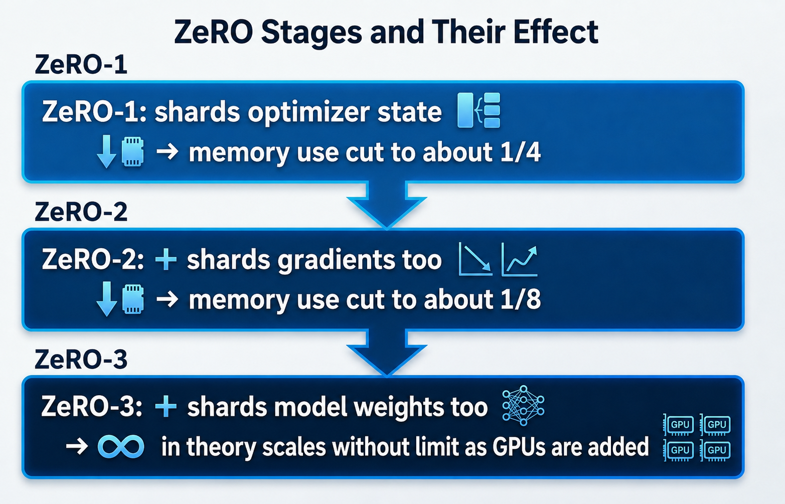
With ZeRO-3, in theory you can train arbitrarily large models by adding more GPUs.
What NVLink Is, and Why It Matters
When GPUs run in parallel for distributed training, they need to exchange data—gradient synchronization, activation transfers, and so on. Huge volumes of data move between GPUs, and the speed of that inter-GPU communication can become the bottleneck.
Normally, GPU-to-GPU communication goes over the PCIe bus. PCIe 4.0 x16, for example, offers about 32GB/s of bandwidth; even PCIe 5.0 only doubles that to 64GB/s.
For large-model training, that is far too slow.
Enter NVLink. NVLink is NVIDIA's high-speed GPU interconnect, with roughly 10x the bandwidth of PCIe.
| Interconnect | Bandwidth | vs. NVLink |
|---|---|---|
| NVLink (H100) | 900 GB/s | 1x |
| NVLink (A100) | 600 GB/s | 0.67x |
| PCIe 5.0 x16 | 64 GB/s | 0.07x |
| 100GbE | 12.5 GB/s | 0.014x |
| 10GbE | 1.25 GB/s | 0.0014x |
Not every GPU can use NVLink, however—and this is an important point.
| GPU | NVLink support | Max GPUs linked |
|---|---|---|
| A6000 / RTX 6000 Ada | ○ | Up to 2 |
| A100 / H100 | ○ | Up to 8 (via NVSwitch) |
| L40S | × | - |
Note that the A6000 and RTX 6000 Ada support NVLink, but only between two cards. With three or more A6000s, NVLink is unavailable and communication falls back to PCIe. The L40S is an Ada Lovelace data-center GPU, but it does not support NVLink at all.
The Multi-Node Communication Bottleneck
Harder still is distributed training that spans multiple servers (nodes).
Within a single server, GPUs can communicate quickly over NVLink or PCIe. Between servers, however, traffic goes over the network. As the table above shows, 10GbE has roughly 1/700 of NVLink's bandwidth, and even 100GbE only about 1/70.
This bandwidth gap imposes major constraints on distributed training design.
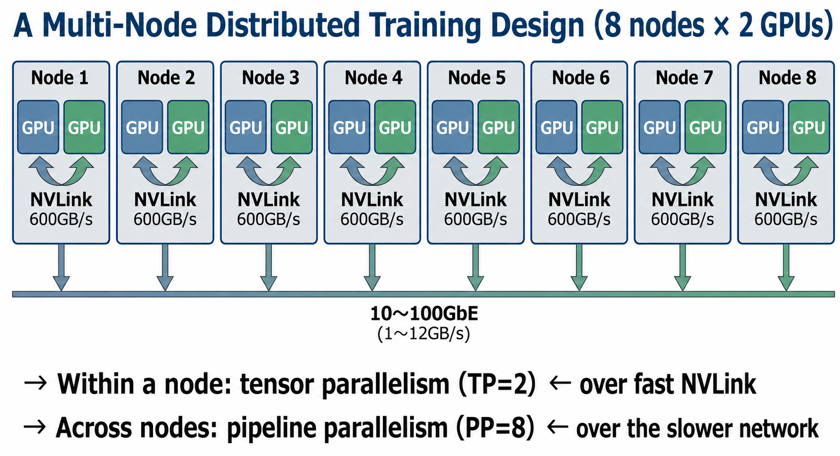
The common design is to keep communication-heavy operations (such as tensor parallelism) within a node over NVLink, and run lower-frequency communication (such as pipeline parallelism) between nodes.
4. How Much Compute LLM Training Requires
What Are Scaling Laws? (2020, OpenAI)
To understand the compute required for LLM training, you need to know the history of scaling laws.
In 2020, OpenAI published the paper "Scaling Laws for Neural Language Models." It showed that a language model's performance (perplexity) depends on three factors—model size, data volume, and compute—and that increasing them improves performance in a predictable way.
Specifically, increasing model size 10x improves performance according to a power law. Increasing data 10x, or compute 10x, improves performance similarly. Crucially, this relationship holds over an astonishingly wide range: the same law applies from tens of millions of parameters to hundreds of billions.
At the time, the paper was widely read as saying "make the model bigger and performance goes up." OpenAI itself followed that course and developed GPT-3 (175 billion parameters).
But there was a problem with that interpretation.
What Is the Chinchilla Law? (2022, DeepMind)
In 2022, DeepMind published "Training Compute-Optimal Large Language Models"—commonly known as the Chinchilla paper.
This paper significantly revised the prevailing interpretation of OpenAI's scaling laws.
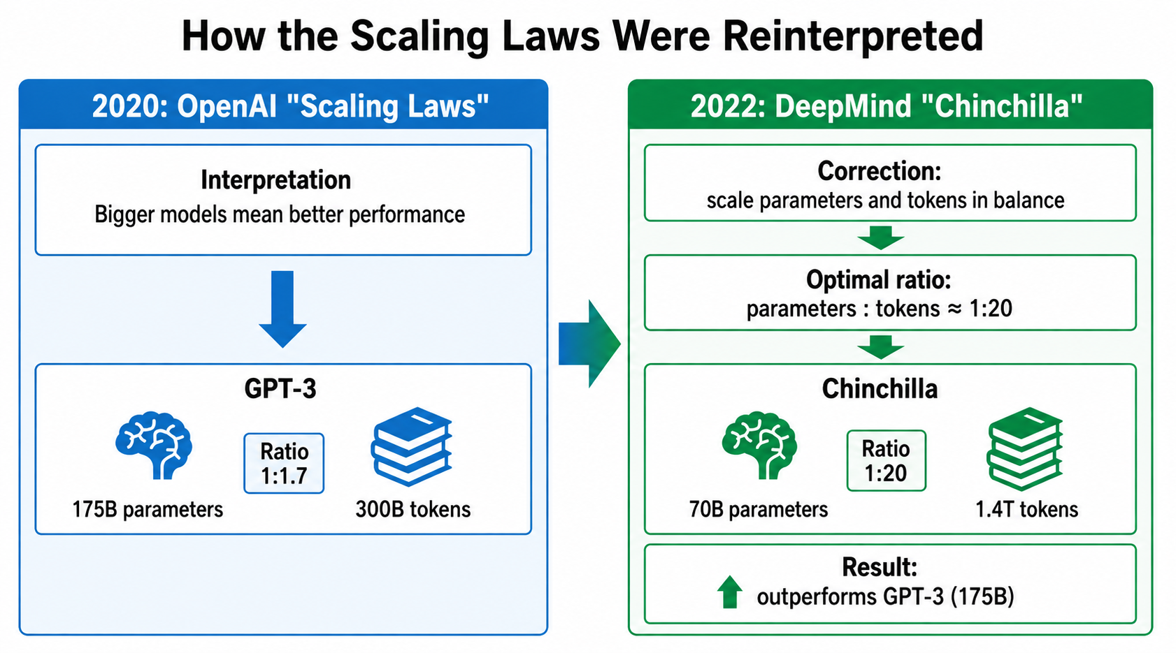
DeepMind's researchers discovered that for a given compute budget, the balance between model size and data volume (token count) is what matters. The optimal ratio is
parameters : tokens ≈ 1 : 20
.
Viewed through this lens, GPT-3 was clearly undertrained: 175 billion parameters trained on only 300 billion tokens. The optimal ratio would have called for around 3.5 trillion tokens.
Based on this theory, DeepMind trained the 70-billion-parameter Chinchilla model on 1.4 trillion tokens. And this 70B model outperformed the 175B GPT-3—with less than half the parameters.
Estimating the Compute Required
The compute needed for LLM training can be roughly estimated with the following formula.
Compute (FLOP) ≈ 6 × parameters × tokens
Why 6? In Transformer training, the forward pass costs about 2x and the backward pass about 4x, for a total of roughly 6x.
Combining this formula with the Chinchilla law reveals something interesting. If you double the model size, the Chinchilla law says you must double the token count as well—so compute quadruples. Compute grows as the square of model size.
| Model size | Optimal tokens | Compute | vs. 10B |
|---|---|---|---|
| 10B | 200B | 1.2×10²² FLOP | 1x |
| 70B | 1.4T | 5.9×10²³ FLOP | 50x |
| 100B | 2T | 1.2×10²⁴ FLOP | 100x |
Optimally training a model 10x larger requires 100x the compute. This square law is why the training cost of large models explodes.
Actual Training Time
Let's convert that compute into actual training time. An A100 80GB has a theoretical BF16 performance of 312 TFLOP/s, but effective performance is around 30–50% of that—roughly 100–150 TFLOP/s.
| Model | Compute | Time on a single A100 |
|---|---|---|
| 10B | 1.2×10²² FLOP | ≈2.5 years |
| 70B | 5.9×10²³ FLOP | ≈125 years |
| 100B | 1.2×10²⁴ FLOP | ≈250 years |
This is why thousands of GPUs become necessary.
Training a 100B model in three months takes roughly 1,000 GPUs.
Even a 100B-class model—not especially large by 2025 standards—requires 1,000 GPUs and three months. That fact alone conveys just how demanding LLM training is.
Very few organizations in Japan can procure GPUs costing millions of yen apiece by the thousand; in practice, the only realistic path is to ride national AI promotion programs.
Needless to say, for individuals or small labs, full-scratch training of an LLM at a genuinely useful scale is close to impossible—that is the reality.
However, the above applies to training completely from scratch. LLM development actually has several other levels of involvement.
5. The Four Levels of LLM Development
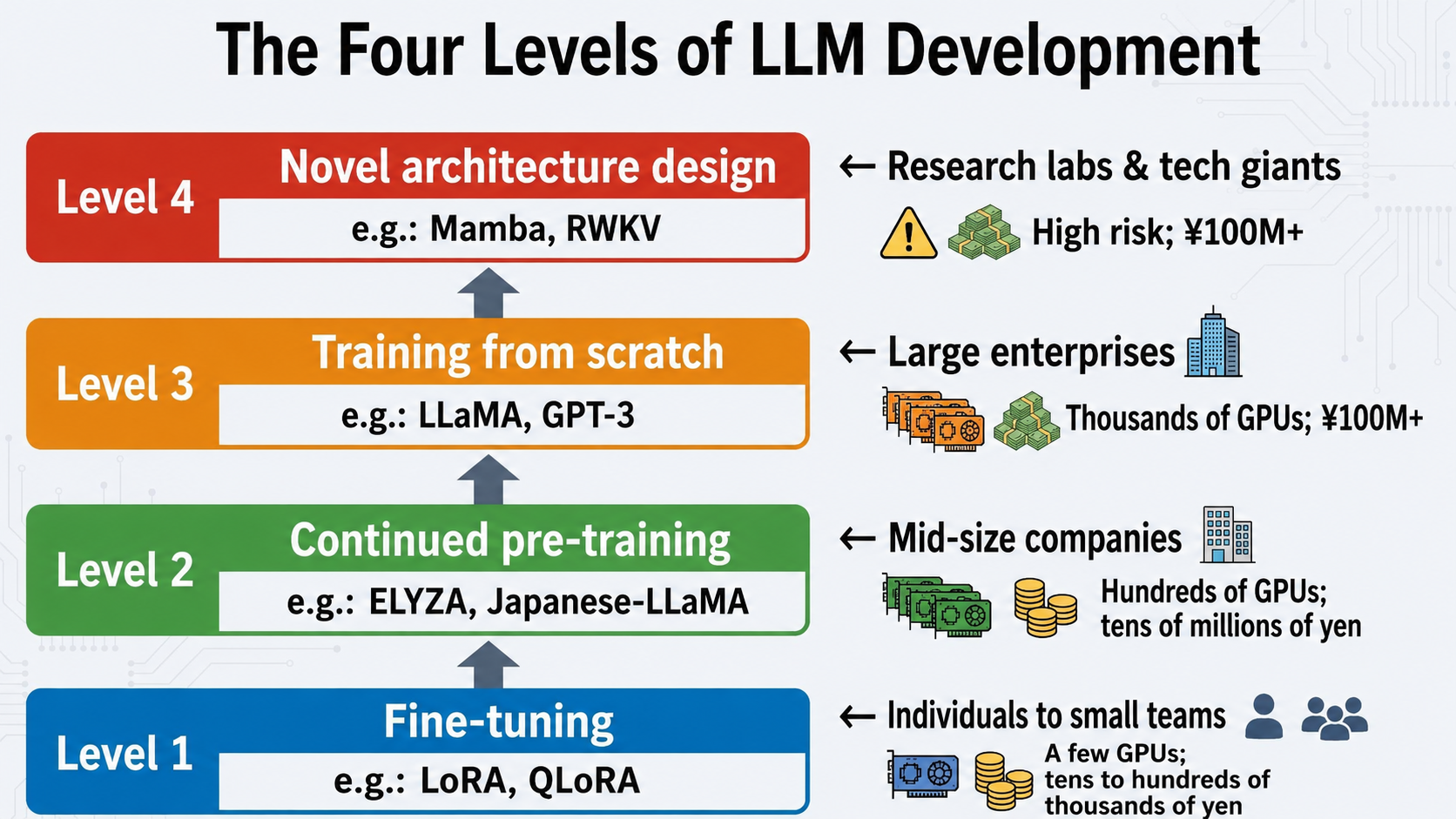
LLM development has four levels, depending on how deep your involvement goes. The required resources and technical difficulty differ enormously between them.
Level 1: Fine-Tuning
The most accessible level is fine-tuning: adapting an existing pre-trained model (LLaMA, Mistral, Qwen, etc.) to a specific task.
What fine-tuning does is adjust the model's behavior: making it respond in chat format, output in a particular structure, or specialize in a specific task (summarization, translation, and so on). It does not substantially change the knowledge the model already has.
The required data is on the order of thousands to tens of thousands of samples. The compute is 1/100 to under 1/1000 of full-scratch training. Techniques like LoRA (Low-Rank Adaptation) and QLoRA (Quantized LoRA) also slash VRAM usage—with QLoRA, you can fine-tune a 70B model on a single 24GB GPU.
Level 2: Continued Pre-Training
The next level is continued pre-training: adding new knowledge or language capability to an existing model.
For example, to add Japanese capability to the English-centric LLaMA, you run continued pre-training on large volumes of Japanese text. Or, to strengthen expertise in a specialized field such as medicine or law, you continue pre-training on documents from that field.
How does this differ from fine-tuning? Where fine-tuning adjusts "behavior," continued pre-training adds "knowledge". The required token count is around 10–20% of full-scratch training.
Level 3: Full-Scratch Training
Full-scratch training means training a model from randomly initialized weights. The training of LLaMA and GPT-3 falls into this category.
The Transformer architecture itself is reused, but the model weights are learned entirely from scratch—everything from the basic structure of language to world knowledge is learned from data.
Per the Chinchilla law, a 100B model needs 2 trillion tokens, or about 1.2×10²⁴ FLOP of compute. Finishing that in three months on H100s takes roughly 1,000 of them.
Level 4: Designing a New Architecture
The most ambitious level is designing a new architecture, as with Mamba or RWKV. Success promises major gains in computational efficiency, but failure can burn hundreds of millions of yen—this is territory for research institutions and large corporations only.
Which Level Should You Choose?
For most organizations, Level 1 (fine-tuning) or Level 2 (continued pre-training) is the realistic choice. With high-performance open models like LLaMA, Mistral, and Qwen freely available, the rationale for training a model from zero is limited.
6. A Detailed Comparison by Training Type
Comparing the Three Training Types
| Item | Fine-tuning | Continued pre-training | Full scratch |
|---|---|---|---|
| Purpose | Adjust behavior | Add knowledge | Learn from zero |
| Data volume | Thousands to tens of thousands of samples | 10–20% of full | Per the Chinchilla law |
| Relative compute cost | 1 | 10–20 | 100 |
| Time for 70B | Hours to days | Weeks | Months (thousands of GPUs) |
| Example uses | Chatbots, task specialization | Adding Japanese, strengthening domain knowledge | Building your own foundation model |
Full-Scratch Training in Detail
Full-scratch training starts from randomly initialized weights. At that point, the model does not even know what language is.
As it reads through massive amounts of training text, the model learns in stages: first word and character patterns, then grammatical structure, then factual knowledge, and finally reasoning ability—all through the simple task of predicting the next word.
Continued Pre-Training in Detail: Why It Needs Less Compute
Why does continued pre-training get away with far less compute than full scratch?
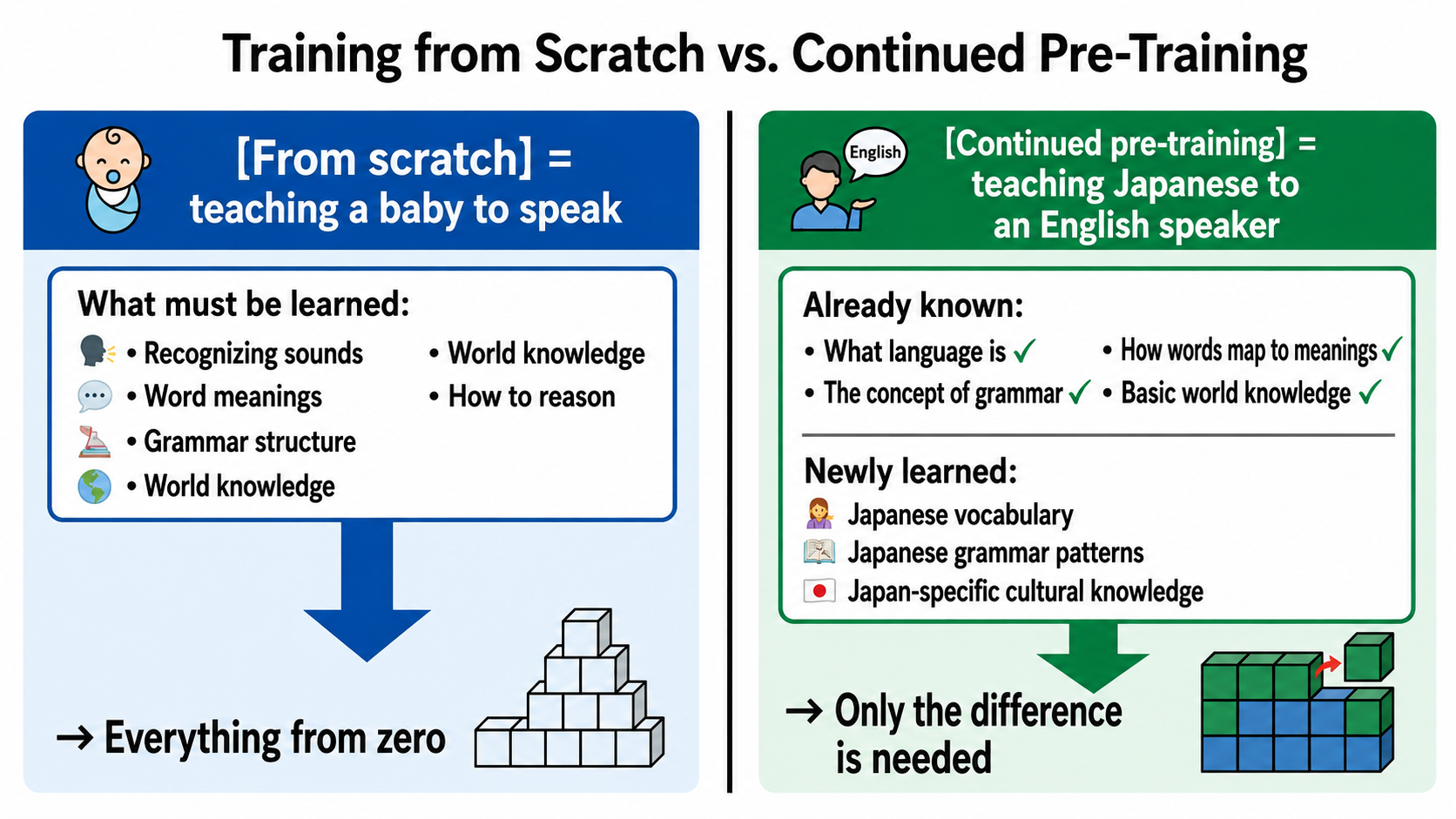
A LLaMA trained on English already knows how to behave as a language model. Continued pre-training in Japanese only needs to learn the Japanese-specific "delta."
In concrete token counts: where a 70B full-scratch run needs 1.4 trillion tokens, continued pre-training delivers results with roughly 100–200 billion—about one-tenth to one-seventh.
One caveat: continued pre-training must avoid erasing the original model's abilities. Training on Japanese alone can degrade its English (catastrophic forgetting), so it is standard practice to mix some English text into the continued pre-training data.
Fine-Tuning in Detail: How LoRA/QLoRA Work
The goal of fine-tuning is not to expand the model's knowledge but to adjust its output format and behavior.
Use LLaMA as-is, for example, and it simply continues the input text. Ask "What is the capital of Japan?" and it might write a continuation of the question—something like "...is a question frequently seen in geography classes." Fine-tuning teaches it the behavior of answering when asked.
LoRA (Low-Rank Adaptation) is a technique that makes fine-tuning efficient.
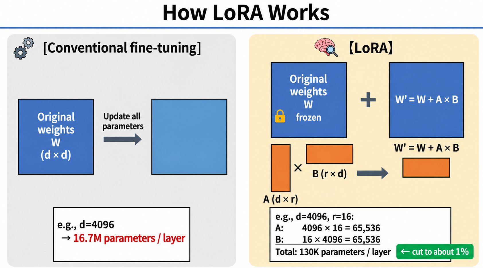
QLoRA takes LoRA a step further: the base model is held in 4-bit quantized form, and only the LoRA adapters are trained in FP16. This makes fine-tuning a 70B model possible with around 24GB of VRAM.
7. How MoE (Mixture of Experts) Works
What Is MoE?
No, not the champagne. In the LLM world, MoE refers to the Mixture of Experts architecture.
Mixtral 8x7B and DeepSeek-V3, among others, adopt it.
The core idea of MoE is that you do not need to use the entire model for every input. Depending on the input, only part of the model is used.
The MoE concept itself is old: it was proposed in 1991 by Jacobs and Hinton (yes, the Hinton who won the 2024 Nobel Prize in Physics). In 2017, Shazeer and colleagues at Google applied it to Transformers, and from 2023 to 2024 the success of Mistral's Mixtral and DeepSeek pushed it firmly into the mainstream.
The Structure of MoE
In a standard Transformer, each layer has an "Attention → FFN" structure. In an MoE Transformer, the FFN is replaced by multiple experts (each an FFN), and only a subset of experts is selected for each input.
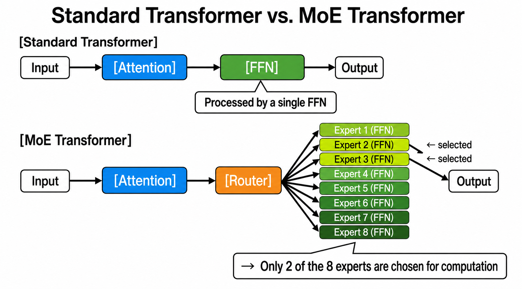
In code, it looks like this.
class MoE(nn.Module):
    def __init__(self, hidden_size, num_experts=8):
        super().__init__()
        # Experts = multiple ordinary FFNs (fully connected layers)
        self.experts = nn.ModuleList([
            nn.Sequential(
                nn.Linear(hidden_size, hidden_size * 4),
                nn.GELU(),
                nn.Linear(hidden_size * 4, hidden_size)
            ) for _ in range(num_experts)
        ])
        # Router = the layer that decides which experts to use
        self.router = nn.Linear(hidden_size, num_experts)

    def forward(self, x):
        scores = self.router(x)  # the router produces scores
        top2_scores, top2_indices = scores.topk(2, dim=-1)  # select the top 2
        # compute with only the selected experts...
Why MoE Reduces Compute
MoE's breakthrough is decoupling parameter count from compute.
| Model | Total params | Active params | Effective compute cost |
|---|---|---|---|
| Dense 70B | 70B | 70B | 70B |
| Mixtral 8x7B | 47B | 13B | 13B |
| DeepSeek-V3 | 671B | 37B | 37B |
Take DeepSeek-V3: it has 671 billion total parameters, but only 37 billion are activated per token. Its compute cost matches a 37B dense model, while the model as a whole carries the "knowledge capacity" of 671 billion parameters.
But VRAM Does Not Shrink
Here is an important caveat: MoE reduces compute, but it does not reduce VRAM usage.
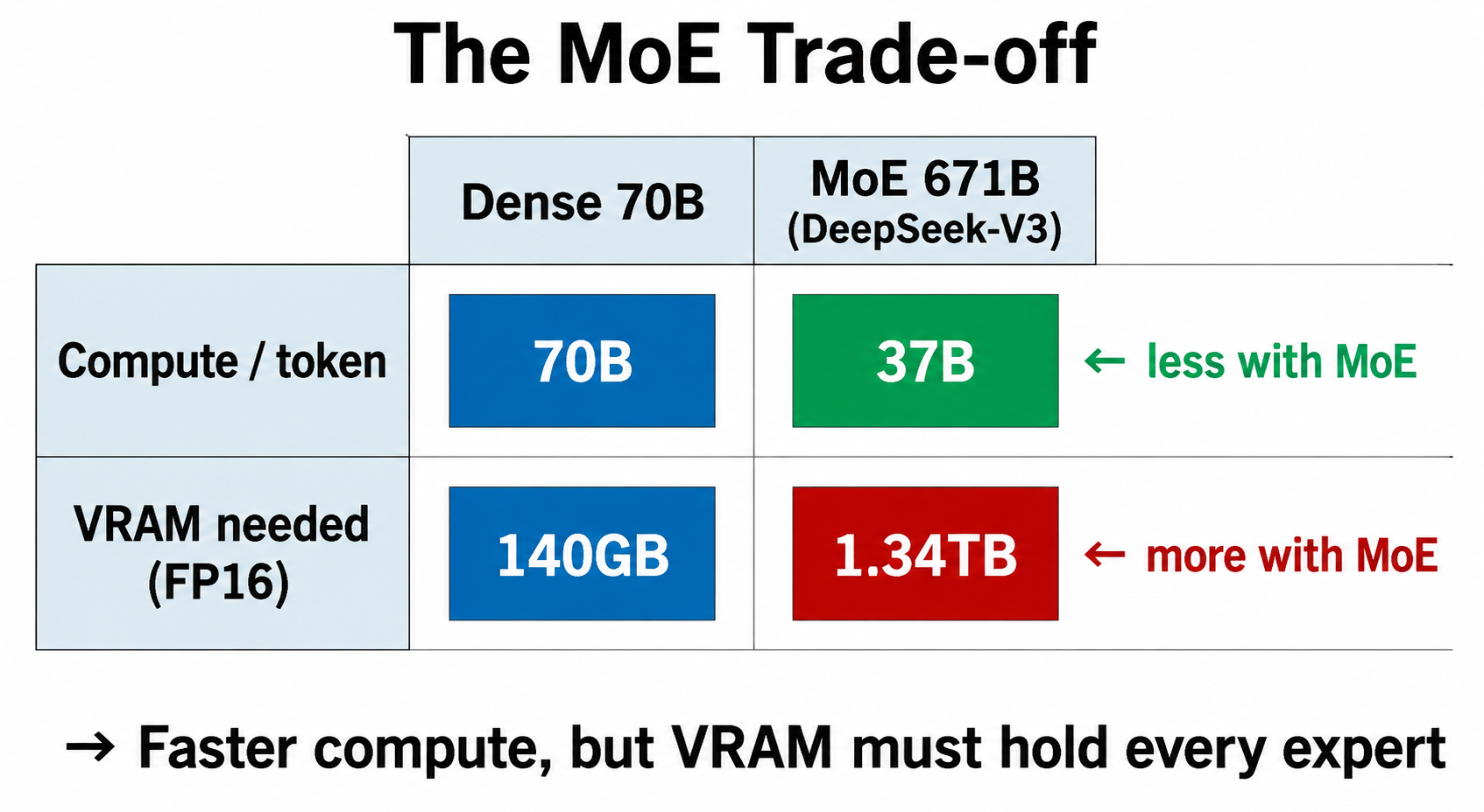
Which experts activate at inference time is decided dynamically based on the input, so all experts must be resident in VRAM.
Why DeepSeek-V3 Is So Cost-Efficient
DeepSeek-V3 trained its 671-billion-parameter MoE model on 2,048 H800s in about two months for roughly $5.6 million (about 800 million yen)—astonishingly cheap for a model of that scale. Why?
| Technique | Effect |
|---|---|
| MoE architecture | Cuts compute to ~1/18 (671B → effectively 37B) |
| FP8 training | Halves compute and communication volume |
| Multi-head Latent Attention | Reduces KV-cache memory |
| Optimized communication patterns | More efficient inter-expert routing |
It combines multiple innovations beyond the MoE architecture itself: FP8 training, Multi-head Latent Attention (MLA), and optimized communication patterns. The know-how accumulated in the roughly nine months since earlier MoE models (such as DBRX) likely contributed significantly as well.
8. Cost Reality from Actual Training Runs
That was a lot of theory. So how much in resources and cost does real LLM training actually consume? Let's look at the publicly available figures.
Training Specs of Past LLMs
The data is somewhat dated, but here are the training scales of LLMs whose figures have been published (some estimated).
| Model | Size | GPU | Count | Duration | Tokens | Cost |
|---|---|---|---|---|---|---|
| LLaMA 2 7B | 7B | A100 80GB | - | 184K GPU-hours | 2T | ≈¥85M |
| LLaMA 2 70B | 70B | A100 80GB | 2,048 | 23 days | 2T | ≈¥500M |
| DBRX | 132B (MoE) | H100 | 3,072 | 2.5 months | 12T | ≈¥1.5B |
| DeepSeek-V3 | 671B (MoE) | H800 | 2,048 | 2 months | 14.8T | ≈¥800M |
| GPT-4 (est.) | ~1.8T (MoE) | - | ~25,000 | 3–5 months | - | ≈¥15B |
*Costs are rough estimates converted to cloud pricing.
LLaMA 2 (Meta, 2023)
LLaMA 2 is the open-source LLM Meta released in 2023. Training the 70B model used 2,048 A100 80GBs for about 23 days. In GPU-hours, that is 2,048 × 24 × 23 ≈ 1.13 million.
At a cloud rate of $3 per A100 80GB hour, 1.13 million × 3 comes to about $3.4 million (roughly 500 million yen).
DBRX vs DeepSeek-V3
Comparing the two is instructive.
| Item | DBRX | DeepSeek-V3 | Ratio |
|---|---|---|---|
| Parameters | 132B | 671B | 5.1x |
| Tokens | 12T | 14.8T | 1.2x |
| GPU count | 3,072 | 2,048 | 0.67x |
| Duration | 2.5 months | 2 months | 0.8x |
| Cost | ≈¥1.5B | ≈¥800M | 0.53x |
DeepSeek-V3 has five times the parameters of DBRX at roughly half the cost. Innovations such as FP8 training and MLA make the difference.
Rules of Thumb for Training Cost
From these examples, we can derive rules of thumb for full-scratch training of dense models: roughly 1,000 GPU-weeks per billion parameters, and roughly ¥7 million per billion parameters. Note that these estimates assume the Chinchilla-optimal amount of training.
9. Realistic Training Scale by GPU
So what can you actually do with which GPU? Let's look at each GPU's specs and its realistic uses.
GPU Spec Comparison
Here are the specs of the GPUs mentioned in this article.
| GPU | VRAM | BF16 performance | Price (approx.) | NVLink |
|---|---|---|---|---|
| A6000 | 48GB | 38 TFLOP/s | ¥700K | Up to 2 |
| A100 40GB | 40GB | 312 TFLOP/s | ¥1M (used) | Up to 8 |
| A100 80GB | 80GB | 312 TFLOP/s | ¥1.8M (used) | Up to 8 |
| H100 SXM | 80GB | 990 TFLOP/s | ¥5M | Up to 8 |
| B200 | 192GB | 2,250 TFLOP/s | From ¥7M | Up to 8 |
You can find details on other GPUs in another article on our blog.
With an A6000 (48GB)
The A6000 is NVIDIA's professional-grade GPU. The caveat is that NVLink connects at most two cards; with three or more, inter-GPU communication goes over PCIe.
| Use | Feasible with 4× A6000? | Notes |
|---|---|---|
| 70B inference (INT4) | ○ | Needs 35GB; ample headroom |
| 70B fine-tuning (QLoRA) | ○ | Possible at ~24GB per GPU |
| 10B continued pre-training | ○ | Takes several weeks |
| 10B full scratch | △ | Months to a year |
| 70B full scratch | × | Unrealistic |
With an A100 (80GB)
The A100 supports NVLink for up to eight GPUs via NVSwitch.
| Use | Feasible with 8× A100 80GB? | Notes |
|---|---|---|
| 70B inference (FP16) | ○ | Needs 140GB; multiple instances possible |
| 70B fine-tuning | ○ | Comfortable |
| 30B continued pre-training | ○ | Several weeks |
| 30B full scratch | ○ | Several months |
| 100B full scratch | × | Takes over a year |
With H100s
The H100 delivers roughly three times the performance of the A100.
| Configuration | What it enables |
|---|---|
| 8× H100 | 3x faster than 8× A100; 30B full scratch becomes realistic |
| 100× H100 | 100B full scratch possible in about 3 months |
| 1,000× H100 | 100B in weeks; still short of GPT-4 class |
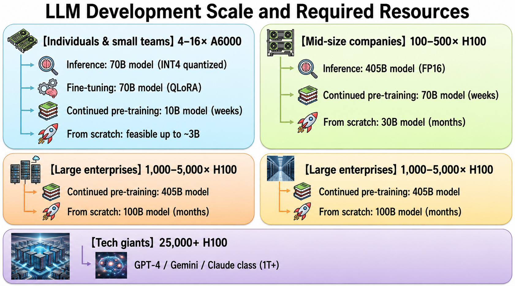
Summary by Scale
10. GPUs for Inference
We do not cover inference in this article, but this series covers it in detail.
11. The State of Japanese LLMs
Let's also take a look at trends in Japanese LLM development.
Japanese open models first appeared around the summer of 2023. As I recall, rinna led the way among Japanese-made models, followed shortly by CyberAgent's. Japanese models likewise began with full-scratch training on architectures based on GPT-NeoX, then shifted to continued pre-training models in the second half of 2023. From 2024 onward, this evolved into continued pre-training on top of the higher-performing Qwen. For the latest high-performance Japanese LLMs, this article presents Japanese LLMs in ranking format.
The Evolution of Japanese LLM Development
| Period | Dominant approach | Representative models |
|---|---|---|
| 2022 to early 2023 | Full scratch | rinna 3.6B, OpenCALM-7B, Weblab-10B |
| Late 2023 onward | Continued pre-training | ELYZA-Llama, Japanese StableLM |
| 2024 onward | Qwen-based | Qwen-derived models from various companies |
Why the Shift from Full Scratch to Continued Pre-Training?
The release of LLaMA in February 2023 was the turning point.
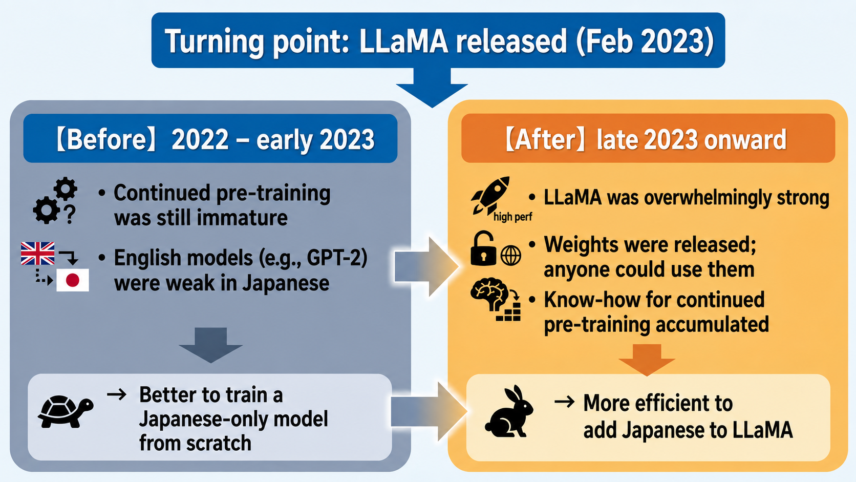
The shift to continued pre-training happened because of efficiency. LLaMA already has the fundamental capabilities of a language model. It became clear that adding Japanese to LLaMA yields higher performance than learning Japanese from zero, at the same compute cost.
Why Qwen-Based Models Are Strong in Japanese
More recently, Japanese models built on Qwen—developed by China's Alibaba—have appeared. Interestingly, Qwen-based models sometimes outperform LLaMA-based ones in Japanese. Why?
The answer lies in the tokenizer.
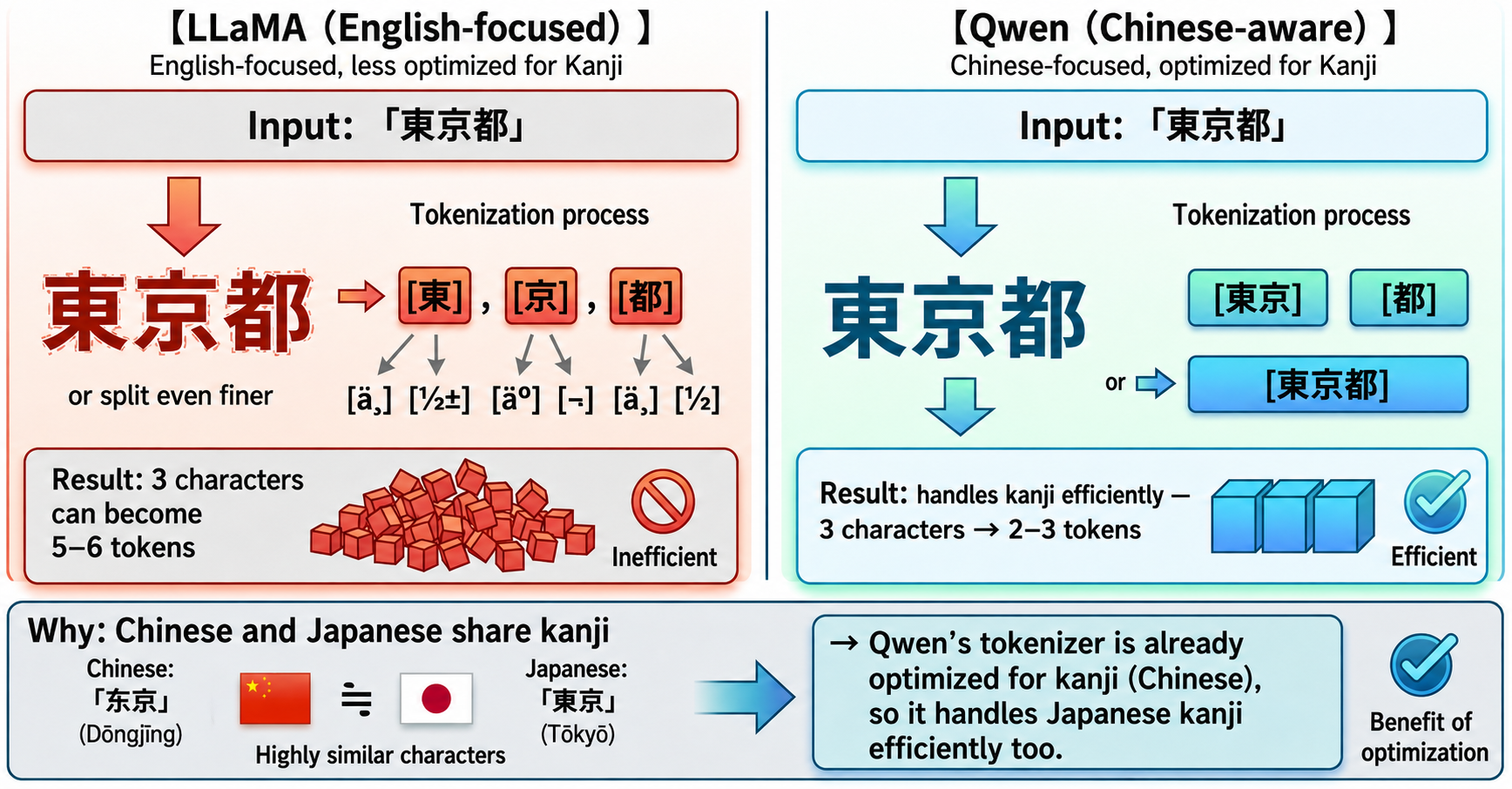
Better token efficiency means more information fits in the same context length. It also lowers the number of tokens needed to train on the same text, improving training efficiency.
Furthermore, Chinese and Japanese share some grammatical structure—the ordering of kanji compounds, polite forms akin to honorifics—making them closer to each other than to English. Adding Japanese to a Chinese model is thought to transfer better than adding it to an English model.
12. Conclusion
Comparison by Training Type
full scratch > continued pre-training > fine-tuning—we have walked through this spectrum of training types, and hopefully it is now clear that in most cases, continued pre-training is more than enough.
| Item | Fine-tuning | Continued pre-training | Full scratch |
|---|---|---|---|
| Purpose | Adjust behavior | Add knowledge | Learn from zero |
| Data volume | Thousands to tens of thousands of samples | 10–20% of full | Parameters × 20 tokens |
| Relative compute cost | 1 | 10–20 | 100 |
| Time for 70B | Hours to days (a few GPUs) | Weeks (hundreds of GPUs) | Months (thousands of GPUs) |
| Example uses | Chatbots, task specialization | Adding Japanese, domain knowledge | Your own foundation model |
Actual Training Runs
We have also seen how costs and timelines balloon exponentially as model size grows.
| Model | Size | GPU count | Duration | Cost |
|---|---|---|---|---|
| LLaMA 2 7B | 7B | - | 184K GPU-hours | ≈¥85M |
| LLaMA 2 70B | 70B | 2,048 | 23 days | ≈¥500M |
| DBRX | 132B (MoE) | 3,072 | 2.5 months | ≈¥1.5B |
| DeepSeek-V3 | 671B (MoE) | 2,048 | 2 months | ≈¥800M |
| GPT-4 (est.) | ~1.8T (MoE) | ~25,000 | 3–5 months | ≈¥15B |
The Bottom Line
As we have seen, full-scratch LLM training is an extremely specialized workload requiring thousands of GPUs and an investment of hundreds of millions to tens of billions of yen. Only a very small number of players in the world can realistically undertake it.
But that does not mean GPU-based LLM development is pointless.
As this article has shown, fine-tuning and continued pre-training are entirely within reach on realistic GPU resources.
With QLoRA, you can fine-tune a 70B model on a single 24GB GPU; with a few A100s, you can add Japanese capability or domain knowledge through continued pre-training. Taking high-performance open models like LLaMA, Mistral, or Qwen as a base and customizing them to your needs—this is the most cost-effective way to put GPUs to work.
On the other hand, not every use case needs GPUs at all. Commercial APIs like ChatGPT and Claude deliver state-of-the-art performance with no infrastructure to manage. For prototyping and small-scale deployments, starting with an API is a perfectly rational choice.
In the end, what matters is not building your own model, but how you put models to use. How will you combine them with your company's own data? Which business processes will you embed them in? What customer value will you create? Whether you customize open models or leverage commercial APIs, that is where differentiation comes from.
Consulting on LLM Adoption and GPU Environments
We hope you found this deep dive useful.
Our company provides hands-on support spanning GPU cluster design and construction, model development in PyTorch, and LLM inference, training, and implementation—grounded not just in theory but in technical validation on our own GPU environment.
"We can't tell which GPU configuration is right for us." "We'd like to try fine-tuning an open model."
"We can't decide between a commercial API and on-premises."
"We want to use open models, but how do we put them to work internally?"
If any of these sound familiar, please feel free to contact us.
GPU selection and training costs—talk to us from the estimation stage.
With GPUs and inference, the challenges never stop—getting things running is hard, and what comes after is harder.
We operate our own GPU clusters and build LLM products. From GPU selection to inference optimization (quantization, vLLM) and distributed configurations, we offer practical advice grounded in real operational experience.
Explore our LLM infrastructure and platform services →References
- Kaplan et al. (2020). "Scaling Laws for Neural Language Models". OpenAI.
- Hoffmann et al. (2022). "Training Compute-Optimal Large Language Models". DeepMind.
- Hu et al. (2021). "LoRA: Low-Rank Adaptation of Large Language Models".
- Dettmers et al. (2023). "QLoRA: Efficient Finetuning of Quantized LLMs".