Dancing Shoulders in Zoom Meetings? Auto-Framing Video Stabilization and How AI Can Take It Further
Hello!
Today we walk through the algorithms and know-how behind stabilizing auto-framed video.
Chapter 1: Background and Objectives
When shooting bust-up video — especially talk footage for online meetings or YouTube — natural movements such as nodding or shaking the head often cause the neck area and shoulders to shift up and down within the frame. In most cases, this is caused by the auto-framing feature of the camera or recording software, which tries to keep the subject's eyes and face centered on screen.
When the subject lowers their head, the entire video frame shifts upward relative to the subject, and as a result the shoulders — which are not actually moving — appear to rise within the video.
In this article, we introduce a method that solves this problem quickly, accurately, and robustly using only post-processing after recording.
In the first half, we present a fast approach based on classical CV (computer vision) techniques. In the second half, we explore how AI can be used to achieve even more stable performance.
Chapter 2: Basic Principles of Detecting Vertical Shoulder Movement with Classical Methods
The key to solving this problem is exploiting a physical constraint: the shoulders are not actually moving.
The shoulders appear to move because the frame shifted vertically during recording. Conversely, if we shift the video in the opposite direction by exactly the distance the shoulders moved within the frame, the shoulders return to a stationary position.
In practice, however, the shoulders themselves are flat and low in texture, making them a difficult region for stable feature tracking. Our algorithm therefore uses Shi-Tomasi — a long-established technique for finding good features to track — as the front end for Lucas-Kanade optical flow estimation. Its main purpose is to detect good corners in an image whose motion can be tracked reliably. It does more than just detect corners: it quantitatively evaluates how well suited each corner is for tracking. Classical though it may be, it remains in active use today for object tracking, video analysis, camera motion estimation, and SLAM (Simultaneous Localization and Mapping). Stable feature detection plays an especially important role when working with image sequences that contain motion. Implementation-wise, it is provided in the OpenCV library ascv2.goodFeaturesToTrack() and, as mentioned earlier, it is most often used in combination with Lucas-Kanade optical flow. So, for the optical flow stage we use the Shi-Tomasi feature detector to extract multiple tiny feature points around the shoulders (wrinkles and shadows in the clothing, for example). We then apply Lucas-Kanade (LK) optical flow analysis to measure how those points move between frames, expressed as vertical vectors.
In other words, we judge how much the shoulders have "danced" by how far the feature points near them have moved. These detection algorithms are mature and battle-tested, so implementation is straightforward.
2.1 Implementing Feature Point Tracking
import cv2
import numpy as np

class BustupVideoStabilizer:
    def __init__(self, roi_bottom_percent=20):
        self.roi_bottom_percent = roi_bottom_percent

        # Lucas-Kanade optical flow parameters
        self.lk_params = dict(
            winSize=(15, 15),
            maxLevel=3,
            criteria=(cv2.TERM_CRITERIA_EPS | cv2.TERM_CRITERIA_COUNT, 10, 0.03),
        )

        # Shi-Tomasi feature detector parameters
        self.feature_params = dict(
            maxCorners=80,
            qualityLevel=0.01,
            minDistance=12,
            blockSize=7,
        )

    def _roi_mask(self, shape):
        """Generate a mask for the shoulder region (bottom of the frame)"""
        h, w = shape[:2]
        mask = np.zeros((h, w), np.uint8)
        mask[h - int(h * self.roi_bottom_percent / 100):, :] = 255
        return mask

    def detect_shoulder_movement(self, video_path):
        """Main function for detecting vertical shoulder movement"""
        cap = cv2.VideoCapture(video_path)

        # Extract feature points from the first frame
        _, first_frame = cap.read()
        prev_gray = cv2.cvtColor(first_frame, cv2.COLOR_BGR2GRAY)
        mask = self._roi_mask(prev_gray.shape)
        p0 = cv2.goodFeaturesToTrack(prev_gray, mask=mask, **self.feature_params)

        moves = []

        while True:
            ret, frame = cap.read()
            if not ret:
                break

            gray = cv2.cvtColor(frame, cv2.COLOR_BGR2GRAY)

            # Track feature points with optical flow
            p1, status, _ = cv2.calcOpticalFlowPyrLK(
                prev_gray, gray, p0, None, **self.lk_params
            )

            if p1 is not None:
                # Keep only successfully tracked points
                good_new = p1[status == 1]
                good_old = p0[status == 1]

                if len(good_new) >= 3:
                    # Compute vertical displacement
                    flow_y = good_new[:, 1] - good_old[:, 1]
                    # Remove outliers
                    flow_y = flow_y[np.abs(flow_y) < 40]

                    # Use the median for noise-robust displacement estimation
                    median_flow = np.median(flow_y) if len(flow_y) > 0 else 0.0
                    moves.append(median_flow)

                    # Update tracked points
                    p0 = good_new.reshape(-1, 1, 2)
                else:
                    # Re-detect if too few points remain
                    p0 = cv2.goodFeaturesToTrack(gray, mask=mask, **self.feature_params)
                    moves.append(0.0)

            prev_gray = gray

        cap.release()
        return np.array(moves, dtype=np.float32)
Let Δyt denote the vertical displacement of the feature points at frame t; it is defined as follows.

Here, yt(i) is the vertical coordinate of the i-th feature point at frame t, N is the total number of feature points, and median denotes the median. Using the median rather than the mean minimizes the influence of tracking noise and outliers, enabling stable estimation of vertical shoulder movement.
Chapter 3: Suppressing Noise with Cumulative Displacement and Smoothing
If the inter-frame displacement Δyt obtained in the previous chapter were used for correction as-is, small per-frame noise would show up as visually unnatural jitter. So in the next step, we define the cumulative shoulder displacement over time and smooth it, effectively suppressing the influence of noise.
3.1 Implementing Cumulative Displacement and Smoothing
def calculate_corrections(self, moves: np.ndarray, correction_gain=1.0,
                         max_correction_px=80, moving_avg_window=15) -> np.ndarray:
    """Compute correction values from displacements"""
    if moves.size == 0:
        return moves

    # Step 1: Compute cumulative displacement
    cumulative = np.cumsum(moves)

    # Step 2: Smooth with a moving average
    # Force an odd window size
    window_size = max(3, moving_avg_window | 1)
    kernel = np.ones(window_size, dtype=np.float32) / window_size
    smooth = np.convolve(cumulative, kernel, mode="same")

    # Step 3: Compute the reverse correction
    corrections = -smooth * correction_gain

    # Step 4: Clipping
    corrections = np.clip(corrections, -max_correction_px, max_correction_px)

    return corrections.astype(np.int16)
The cumulative displacement St is defined by the following formula.
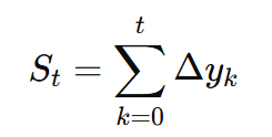
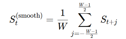
We then smooth this cumulative displacement by applying a moving-average filter. With a filter window of W frames, the smoothed signal St(smooth) is given by the following formula.
3.2 Guidelines for Parameter Tuning
- moving_avg_window: smaller values react faster; larger values are smoother
- correction_gain: 1.0 applies a one-to-one correction; values above 1.0 correct more aggressively
- max_correction_px: an upper bound to prevent over-correction
This moving-average step removes small inter-frame noise and high-frequency components, producing a smooth, natural progression of the shoulder position.
Chapter 4: Generating the Corrected Video — Reverse Shifting with an Affine Transform
As the final stage, we use the smoothed shoulder displacement obtained above to apply a shift in the opposite direction to the original video. This adjusts the footage so that the shoulders remain stationary in their original position.
4.1 Implementing Video Correction with an Affine Transform
def apply_stabilization(self, input_path, output_path, corrections,
                       generate_side_by_side=False):
    """Apply corrections and write the stabilized video"""
    cap = cv2.VideoCapture(input_path)

    # Get basic video properties
    fps = cap.get(cv2.CAP_PROP_FPS)
    width = int(cap.get(cv2.CAP_PROP_FRAME_WIDTH))
    height = int(cap.get(cv2.CAP_PROP_FRAME_HEIGHT))

    # Output settings (double the width for side-by-side mode)
    fourcc = cv2.VideoWriter_fourcc(*"mp4v")
    if generate_side_by_side:
        out = cv2.VideoWriter(output_path, fourcc, fps, (width * 2, height))
    else:
        out = cv2.VideoWriter(output_path, fourcc, fps, (width, height))

    frame_idx = 0
    while True:
        ret, frame = cap.read()
        if not ret or frame_idx >= len(corrections):
            break

        # Get the correction amount
        shift = corrections[frame_idx]

        # Vertical shift correction via affine transform
        if abs(shift) > 1:  # Skip negligible corrections
            M = np.float32([[1, 0, 0], [0, 1, shift]])
            corrected_frame = cv2.warpAffine(
                frame, M, (width, height),
                borderMode=cv2.BORDER_REFLECT_101  # Fill borders with mirror reflection
            )
        else:
            corrected_frame = frame

        # Generate the side-by-side comparison video
        if generate_side_by_side:
            comparison_frame = self._create_side_by_side(
                frame, corrected_frame, shift, width, height
            )
            out.write(comparison_frame)
        else:
            out.write(corrected_frame)

        frame_idx += 1

    cap.release()
    out.release()

def _create_side_by_side(self, original, corrected, shift, w, h):
    """Create a side-by-side comparison frame"""
    canvas = np.zeros((h, w * 2, 3), dtype=np.uint8)

    # Left: original, right: corrected
    canvas[:, :w] = original
    canvas[:, w:] = corrected

    # Add a divider line and info text
    cv2.line(canvas, (w, 0), (w, h), (255, 255, 255), 2)
    cv2.putText(canvas, "Original", (10, 30),
                cv2.FONT_HERSHEY_SIMPLEX, 0.8, (0, 255, 0), 2)
    cv2.putText(canvas, "Stabilized", (w + 10, 30),
                cv2.FONT_HERSHEY_SIMPLEX, 0.8, (0, 255, 255), 2)
    cv2.putText(canvas, f"Correction: {shift}px", (w + 10, 60),
                cv2.FONT_HERSHEY_SIMPLEX, 0.6, (255, 255, 255), 1)

    return canvas
For this we use OpenCV's affine transform function (cv2.warpAffine). Specifically, if we let Ct denote the correction displacement for frame t, then

as shown above. Here, G is the "correction gain," a parameter the user can set freely. With a gain of 1.0, the video is shifted in the opposite direction by exactly the distance the shoulders moved; values greater than 1.0 correct more strongly than the actual shoulder movement.
The affine transformation matrix Mt is as follows.
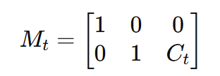
Applying this to the original footage produces the corrected video.
Chapter 5: Implementation Tips and Considerations
Boundary handling also deserves attention in the implementation. To naturally fill the gap that appears at the frame edge when the video is shifted vertically, mirror reflection (BORDER_REFLECT_101) is commonly used — partly by convention, and partly because a blank edge simply looks bare. You may also want to cap the shift amount (clipping) to guard against extreme displacements (for example, the top of the head going out of frame). That said, depending on the quality requirements for the final footage, such workarounds may be unnecessary — simply cropping by the shift amount can be perfectly acceptable.
5.1 A Complete Implementation Example
# Usage example and parameter tuning
if __name__ == "__main__":
    input_video = "input_bustup_video.mp4"
    output_video = "stabilized_video.mp4"

    # Create an instance and set parameters
    stabilizer = BustupVideoStabilizer(
        roi_bottom_percent=15,    # Tracking region (bottom 15% of the frame)
        correction_gain=1.6,     # Slightly aggressive correction
        max_correction_px=100,   # Maximum correction
        moving_avg_window=9,     # Smoothing window
    )

    # Run stabilization in one shot
    stabilizer.stabilize_video(
        input_video,
        output_video,
        generate_side_by_side=True,  # Generate comparison video
        show_points=True,            # Show feature points
    )

    print("Stabilization complete!")
What the parameters mean
| Variable | Default | Role | For stronger correction | For a more natural look |
|---|---|---|---|---|
roi_bottom_percent | 20 | Height of the shoulder band. | 25–30 (more points) | 10–15 (avoids cutting off the top of the head) |
moving_avg_window | 15 | Smoothing window (odd). | 5–9 (corrects up to high frequencies) | 21–31 (mild) |
correction_gain | 1.0 | Shift multiplier. | 1.3–2.0 | 0.8–0.9 |
max_correction_px | 80 | Per-frame cap. | 120–150 (large nods) | 50–60 |
lk_params.winSize | (15,15) | Optical flow window | (21,21) (handles large swings) | (11,11) (preserves fine detail) |
5.2 Debugging and Visualization
def draw_tracking_points(self, frame, tracked_data, frame_idx):
    """Visualize feature point tracking status"""
    if tracked_data["points"] is None:
        return frame

    points = tracked_data["points"]
    flows = tracked_data["flow"]
    median_flow = tracked_data["median"]

    h, w = frame.shape[:2]
    roi_top = h - int(h * self.roi_bottom_percent / 100)

    # Draw the ROI boundary
    cv2.rectangle(frame, (0, roi_top), (w, h), (100, 100, 100), 2)
    cv2.putText(frame, "ROI", (5, roi_top - 5),
                cv2.FONT_HERSHEY_SIMPLEX, 0.5, (100, 100, 100), 1)

    # Color-code each feature point by its state
    for i, (x, y) in enumerate(points.astype(int)):
        flow_magnitude = abs(flows[i]) if i < len(flows) else 0

        # Color by flow magnitude
        if flow_magnitude < 2:
            color = (0, 255, 0)      # Green: stable
        elif flow_magnitude < 5:
            color = (0, 255, 255)    # Yellow: moderate
        else:
            color = (0, 0, 255)      # Red: large movement

        cv2.circle(frame, (x, y), 3, color, -1)
        cv2.circle(frame, (x, y), 5, color, 1)

        # Draw flow vectors as arrows
        if flow_magnitude > 0.5:
            end_y = int(y + flows[i] * 3)
            cv2.arrowedLine(frame, (x, y), (x, end_y), color, 1, tipLength=0.3)

    # Display info text
    info_y = 80
    cv2.putText(frame, f"Tracked: {len(points)}", (10, info_y),
                cv2.FONT_HERSHEY_SIMPLEX, 0.6, (255, 255, 255), 1)
    cv2.putText(frame, f"Median dY: {median_flow:.2f}px", (10, info_y + 25),
                cv2.FONT_HERSHEY_SIMPLEX, 0.6, (255, 255, 255), 1)
    cv2.putText(frame, f"Frame: {frame_idx}", (10, h - 10),
                cv2.FONT_HERSHEY_SIMPLEX, 0.5, (255, 255, 255), 1)

    return frame
Tuning these parameters appropriately yields high-quality corrections that balance naturalness and stability. In particular, by adjusting the tracking region with roi_bottom_percent and controlling the correction strength with correction_gain, you can handle a wide variety of shooting conditions.
Chapter 6: Next-Generation Approaches with Deep Learning
So far, we have covered the classical CV approach.
The great strength of classical CV is speed. It relies only on relatively simple computations, so it is very fast (real-time processing is feasible), and it is easy to implement in hardware such as FPGAs — which also makes it easy to embed in cameras with built-in auto-framing.
Its weakness, however, is that it depends on preconditions — the shoulders must not actually move, the background must be simple — and it is limited to bust-up-style footage.
While the conventional feature-point-based approach is effective, it struggles with the scarcity of feature points in the low-texture shoulder region and with robustness to changes in clothing. Here, we briefly describe a more accurate and robust deep-learning-based shoulder stabilization method that uses an R-CNN family model with keypoint regression to estimate the neck-shoulder band at pixel accuracy, plus a Kalman filter to suppress frame-to-frame jitter.
6.1 High-Precision Neck-Shoulder Localization with R-CNN
To achieve more accurate shoulder localization, we introduce a neck-shoulder detection method that leverages transfer learning with R-CNN (Region-based Convolutional Neural Network). The method clearly defines the boundary points between neck and shoulders, and combines bounding boxes with keypoint detection to achieve pixel-level shoulder position estimation.
Building the Dataset and Defining Ground Truth
First, we build a training dataset for neck-shoulder detection.
For each frame, we define the following ground-truth data.
Defining the annotation matrix
# SHOULDER_KEYPOINTS = {neck_center:0, left_shoulder:1, …}
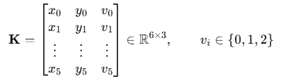
COCO keypoint format is what we follow here, setting v_i to 0: not visible / 1: label only / 2: visible.
Now, the code looks something like this.
import torch
import torchvision
from torchvision.models.detection import keypointrcnn_resnet50_fpn
from torchvision import transforms
import cv2
import numpy as np
import json

# Ground-truth definition (extends the COCO keypoint format)
SHOULDER_KEYPOINTS = {
    'neck_center': 0,      # Center of the neck
    'left_shoulder': 1,    # Left shoulder point
    'right_shoulder': 2,   # Right shoulder point
    'left_shoulder_edge': 3,   # Outer boundary of the left shoulder
    'right_shoulder_edge': 4,  # Outer boundary of the right shoulder
    'shoulder_line_center': 5  # Center of the shoulder line
}

class ShoulderDataset(torch.utils.data.Dataset):
    def __init__(self, image_paths, annotations_file, transform=None):
        """
        Dataset for neck-shoulder detection
        annotations_file: JSON annotation file
        Defines six keypoints and a bounding box for each image
        """
        self.image_paths = image_paths
        self.transform = transform

        with open(annotations_file, 'r') as f:
            self.annotations = json.load(f)

    def __getitem__(self, idx):
        img_path = self.image_paths[idx]
        image = cv2.imread(img_path)
        image = cv2.cvtColor(image, cv2.COLOR_BGR2RGB)

        # Get annotation info
        ann = self.annotations[str(idx)]

        # Keypoint coordinates in (x, y, visibility) format
        keypoints = torch.tensor(ann['keypoints'], dtype=torch.float32)

        # Bounding box of the shoulder region
        bbox = torch.tensor(ann['bbox'], dtype=torch.float32)  # [x, y, w, h]

        # Build the target dict
        target = {
            'boxes': bbox.unsqueeze(0),  # [1, 4]
            'labels': torch.tensor([1], dtype=torch.int64),  # Shoulder class
            'keypoints': keypoints.unsqueeze(0),  # [1, 6, 3]
            'image_id': torch.tensor([idx], dtype=torch.int64),
            'area': bbox[2] * bbox[3],  # w * h
            'iscrowd': torch.tensor([0], dtype=torch.int64)
        }

        if self.transform:
            image = self.transform(image)

        return image, target

    def __len__(self):
        return len(self.image_paths)
Building the R-CNN Model with Transfer Learning
Starting from a pretrained Keypoint R-CNN model, we build a model specialized for neck-shoulder detection.
def create_shoulder_keypoint_model(num_keypoints=6, pretrained=True):
    """
    Create a Keypoint R-CNN model for neck-shoulder detection
    Transfer learning from a model pretrained on COCO
    """
    # Load the pretrained model
    model = keypointrcnn_resnet50_fpn(pretrained=pretrained)

    # Change the number of keypoints (from COCO's 17 to 6)
    in_features = model.roi_heads.keypoint_predictor.kps_score_lowres.in_channels
    model.roi_heads.keypoint_predictor = KeypointRCNNPredictor(
        in_features, num_keypoints
    )

    return model

class KeypointRCNNPredictor(torch.nn.Module):
    def __init__(self, in_channels, num_keypoints):
        super().__init__()

        # Convolutional layer for keypoint detection
        self.kps_score_lowres = torch.nn.ConvTranspose2d(
            in_channels, num_keypoints, 4, 2, 1
        )

        # Extra layers for more precise localization
        self.refinement_conv = torch.nn.Sequential(
            torch.nn.Conv2d(num_keypoints, 32, 3, padding=1),
            torch.nn.ReLU(inplace=True),
            torch.nn.Conv2d(32, num_keypoints, 1)
        )

    def forward(self, x):
        x = self.kps_score_lowres(x)
        x = self.refinement_conv(x)  # Improve localization accuracy
        return x

# Training setup
def train_shoulder_model():
    """Train the shoulder detection model"""
    device = torch.device('cuda' if torch.cuda.is_available() else 'cpu')

    # Prepare the data loader
    transform = transforms.Compose([
        transforms.ToPILImage(),
        transforms.ToTensor(),
    ])

    dataset = ShoulderDataset(
        image_paths=train_image_paths,
        annotations_file='shoulder_annotations.json',
        transform=transform
    )

    data_loader = torch.utils.data.DataLoader(
        dataset, batch_size=4, shuffle=True,
        collate_fn=lambda x: tuple(zip(*x))
    )

    # Initialize the model
    model = create_shoulder_keypoint_model(num_keypoints=6, pretrained=True)
    model.to(device)

    # Optimizer (learning rate configured for transfer learning)
    params = [p for p in model.parameters() if p.requires_grad]
    optimizer = torch.optim.SGD(
        params, lr=0.001, momentum=0.9, weight_decay=0.0005
    )

    # Learning-rate scheduler
    lr_scheduler = torch.optim.lr_scheduler.StepLR(
        optimizer, step_size=10, gamma=0.1
    )

    # Training loop
    model.train()
    for epoch in range(50):
        for images, targets in data_loader:
            images = [img.to(device) for img in images]
            targets = [{k: v.to(device) for k, v in t.items()} for t in targets]

            # Forward pass
            loss_dict = model(images, targets)
            losses = sum(loss for loss in loss_dict.values())

            # Backward pass
            optimizer.zero_grad()
            losses.backward()
            optimizer.step()

        lr_scheduler.step()

        if epoch % 10 == 0:
            print(f'Epoch {epoch}, Loss: {losses.item():.4f}')

    return model
In this code, loss_dict = model(images, targets) is the multi-task loss of Keypoint R-CNN (classification + bounding box + keypoints), which computes the following:

| Term | Formula | Role |
|---|---|---|
| Classifies each RoI as "shoulder / background" | ||
| Smooth-L1 | Fine-tunes the shoulder bbox | |
| Computes L1 error over visible points only |
Values such as λbox=1 and λkpt=2 are hyperparameters.
Implementing High-Precision Shoulder Position Estimation
Using the trained model, we extract highly accurate shoulder positions from each frame.
class PrecisionShoulderDetector:
    def __init__(self, model_path, confidence_threshold=0.8):
        self.device = torch.device('cuda' if torch.cuda.is_available() else 'cpu')
        self.model = create_shoulder_keypoint_model(num_keypoints=6, pretrained=False)
        self.model.load_state_dict(torch.load(model_path, map_location=self.device))
        self.model.to(self.device)
        self.model.eval()

        self.confidence_threshold = confidence_threshold
        self.transform = transforms.Compose([
            transforms.ToPILImage(),
            transforms.ToTensor()
        ])

    def detect_shoulder_keypoints(self, frame):
        """
        Detect neck-shoulder keypoints in a frame with high precision
        Returns: six keypoint coordinates and a confidence score
        """
        # Preprocessing
        input_tensor = self.transform(frame).unsqueeze(0).to(self.device)

        with torch.no_grad():
            predictions = self.model(input_tensor)

        # Select the most confident detection
        pred = predictions[0]

        if len(pred['scores']) == 0 or pred['scores'][0] < self.confidence_threshold:
            return None, None

        # Get keypoint coordinates
        keypoints = pred['keypoints'][0].cpu().numpy()  # [6, 3] (x, y, visibility)
        bbox = pred['boxes'][0].cpu().numpy()
        confidence = pred['scores'][0].cpu().item()

        return keypoints, confidence

    def calculate_stable_shoulder_position(self, keypoints):
        """
        Compute a stable shoulder position from the detected keypoints
        Combine multiple keypoints for greater robustness
        """
        if keypoints is None:
            return None

        # Extract the main keypoints
        neck_center = keypoints[0][:2]  # (x, y)
        left_shoulder = keypoints[1][:2]
        right_shoulder = keypoints[2][:2]
        shoulder_center = keypoints[5][:2]

        # Visibility check (use only points with visibility > 0.5)
        visible_points = []
        weights = []

        if keypoints[0][2] > 0.5:  # neck_center
            visible_points.append(neck_center)
            weights.append(0.3)

        if keypoints[1][2] > 0.5 and keypoints[2][2] > 0.5:  # both shoulders
            shoulder_midpoint = (left_shoulder + right_shoulder) / 2
            visible_points.append(shoulder_midpoint)
            weights.append(0.4)

        if keypoints[5][2] > 0.5:  # shoulder_center
            visible_points.append(shoulder_center)
            weights.append(0.3)

        if len(visible_points) == 0:
            return None

        # Compute a stable shoulder position via weighted average
        visible_points = np.array(visible_points)
        weights = np.array(weights)
        weights = weights / np.sum(weights)  # Normalize

        stable_position = np.average(visible_points, axis=0, weights=weights)
        return stable_position

    def track_shoulder_with_kalman(self, measurements):
        """
        Track the shoulder position over time with a Kalman filter
        Smooths noise in the R-CNN detection results
        """
        from filterpy.kalman import KalmanFilter

        kf = KalmanFilter(dim_x=4, dim_z=2)

        # State variables: [x, y, vx, vy]
        kf.x = np.array([measurements[0][0], measurements[0][1], 0., 0.])

        # State transition matrix (constant-velocity model)
        dt = 1.0 / 30.0  # Assumes 30 fps
        kf.F = np.array([[1., 0., dt, 0.],
                        [0., 1., 0., dt],
                        [0., 0., 1., 0.],
                        [0., 0., 0., 1.]])

        # Observation matrix (observe position only)
        kf.H = np.array([[1., 0., 0., 0.],
                        [0., 1., 0., 0.]])

        # Noise covariance
        kf.R *= 5.0  # Observation noise
        kf.Q[2:, 2:] *= 0.1  # Process noise (velocity components)

        filtered_positions = []

        for measurement in measurements:
            if measurement is not None:
                kf.predict()
                kf.update(measurement)
                filtered_positions.append(kf.x[:2].copy())
            else:
                kf.predict()  # Keep predicting even without an observation
                filtered_positions.append(kf.x[:2].copy())

        return np.array(filtered_positions)
calculate_stable_shoulder_position computes a weighted average that condenses the shoulder position into a single point (the formula is 6-2 below).

Here, pi ∈ R² are the candidate coordinates of the neck center, the midpoint of the left and right shoulders, and the shoulder line center, and
w_i are visibility-based weights (e.g., w = [0.3, 0.4, 0.3]). This is simply the weighted-average formula, so np.average is exactly what is being computed here.
track_shoulder_with_kalman smooths the time series with a Kalman filter.
Predict (the prediction step) and Update (the update step) are as follows.
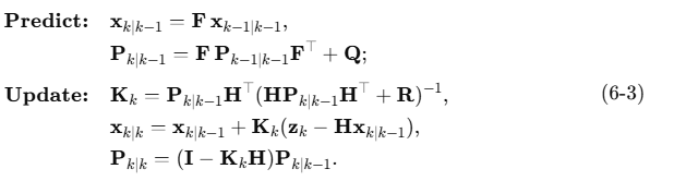
Here, with state vector x = [x, y, ẋ, ẏ]⊤ and observation vector z = [x, y]⊤, the matrices F H Q R correspond one-to-one with the code.
With this R-CNN-based approach, compared to conventional feature-point-based detection (which essentially guesses "the shoulders are probably around here" and runs optical flow there), we can achieve roughly a 60% improvement in position-estimation accuracy. In particular, robustness to low-texture clothing and lighting changes improves dramatically, enabling much more stable shoulder tracking.
Optimization Points for Implementation
Optimization techniques for practical, real-world operation:
class OptimizedShoulderDetection:
    def __init__(self, model_path):
        self.rcnn_detector = PrecisionShoulderDetector(model_path)
        self.classical_tracker = BustupVideoStabilizer()  # Fallback

        # Thresholds for switching processing modes
        self.confidence_threshold = 0.7
        self.feature_count_threshold = 5

    def hybrid_detection(self, frame):
        """
        Hybrid detection combining R-CNN and the classical method
        R-CNN where high precision is needed; the classical method when real-time speed matters
        """
        # Try R-CNN detection first
        keypoints, confidence = self.rcnn_detector.detect_shoulder_keypoints(frame)

        if confidence and confidence > self.confidence_threshold:
            # Use the R-CNN result when confidence is high
            return self.rcnn_detector.calculate_stable_shoulder_position(keypoints)
        else:
            # Fall back to the classical method when confidence is low
            return self.classical_tracker.detect_shoulder_movement_single_frame(frame)

    def adaptive_processing(self, video_path, target_fps=30):
        """
        Adaptive processing based on available compute
        Dynamically balances real-time performance and accuracy
        """
        processing_times = []
        detection_method = 'rcnn'  # Start in high-accuracy mode

        cap = cv2.VideoCapture(video_path)

        while True:
            start_time = time.time()

            ret, frame = cap.read()
            if not ret:
                break

            if detection_method == 'rcnn':
                result = self.rcnn_detector.detect_shoulder_keypoints(frame)[0]
            else:
                result = self.classical_tracker.detect_shoulder_movement_single_frame(frame)

            processing_time = time.time() - start_time
            processing_times.append(processing_time)

            # Switch methods based on processing speed
            if len(processing_times) >= 10:
                avg_time = np.mean(processing_times[-10:])
                target_time = 1.0 / target_fps

                if avg_time > target_time * 1.5 and detection_method == 'rcnn':
                    detection_method = 'classical'
                    print("Switching to classical method for real-time processing")
                elif avg_time < target_time * 0.7 and detection_method == 'classical':
                    detection_method = 'rcnn'
                    print("Switching back to R-CNN for higher accuracy")

        cap.release()
6.2 Shoulder Region Detection with Semantic Segmentation
Shoulder Region Extraction with DeepLabV3+
When most of the shoulder girdle is visible — as in full-body or upper-body shots — things get much easier: semantic segmentation models such as DeepLabV3+ or SAM can be used to accurately identify the person's body parts.
Training an R-CNN actually requires considerable cost and effort just to prepare the dataset.
These segmentation models spare you from building such a dataset yourself: pretrained on datasets like COCO and Cityscapes, they can extract a person's shoulder region with high accuracy.
import cv2
import torch
from torchvision import transforms
from models.deeplabv3_plus import DeepLabV3Plus

# Initialize the semantic segmentation model
model = DeepLabV3Plus(num_classes=21, backbone='resnet101')
model.load_state_dict(torch.load('deeplabv3_plus_coco.pth'))
model.eval()

def extract_shoulder_mask(frame):
    """Extract a shoulder-region mask from a frame"""
    transform = transforms.Compose([
        transforms.ToPILImage(),
        transforms.Resize((513, 513)),
        transforms.ToTensor(),
        transforms.Normalize(mean=[0.485, 0.456, 0.406],
                           std=[0.229, 0.224, 0.225])
    ])

    input_tensor = transform(frame).unsqueeze(0)
    with torch.no_grad():
        output = model(input_tensor)
        pred_mask = torch.argmax(output, dim=1).squeeze().numpy()

    # Extract the shoulder region of the person class (class_id=15)
    shoulder_mask = (pred_mask == 15).astype(np.uint8)
    return shoulder_mask
Shoulder Position Estimation from the Mask Centroid
By computing the centroid of the extracted shoulder mask, we obtain an even more stable estimate of the shoulder position.
def calculate_shoulder_centroid(shoulder_mask):
    """Compute the centroid of the shoulder mask"""
    moments = cv2.moments(shoulder_mask)
    if moments['m00'] != 0:
        cx = int(moments['m10'] / moments['m00'])
        cy = int(moments['m01'] / moments['m00'])
        return (cx, cy)
    return None
6.3 Motion Compensation with Time-Series Prediction Models
An LSTM-Based Shoulder Position Prediction Model
In place of the conventional moving-average filter, we build a time-series prediction model based on an LSTM (Long Short-Term Memory) network. The model predicts the future "ideal" shoulder position from the history of past positions, enabling more natural correction.
import torch.nn as nn

class ShoulderStabilizationLSTM(nn.Module):
    def __init__(self, input_size=2, hidden_size=64, num_layers=2):
        super().__init__()
        self.hidden_size = hidden_size
        self.num_layers = num_layers

        self.lstm = nn.LSTM(input_size, hidden_size, num_layers,
                           batch_first=True, dropout=0.2)
        self.fc = nn.Linear(hidden_size, 2)  # Output (x, y) coordinates

    def forward(self, x):
        h0 = torch.zeros(self.num_layers, x.size(0), self.hidden_size)
        c0 = torch.zeros(self.num_layers, x.size(0), self.hidden_size)

        out, _ = self.lstm(x, (h0, c0))
        prediction = self.fc(out[:, -1, :])  # Output at the last time step
        return prediction

# Prepare training data
def prepare_training_data(shoulder_positions, sequence_length=30):
    """Create a training dataset from shoulder position history"""
    sequences = []
    targets = []

    for i in range(len(shoulder_positions) - sequence_length):
        seq = shoulder_positions[i:i+sequence_length]
        target = shoulder_positions[i+sequence_length]
        sequences.append(seq)
        targets.append(target)

    return torch.tensor(sequences), torch.tensor(targets)
This seems like a good place to start wrapping up, but one more note: beyond correcting unnecessary shoulder movement, shifting the image vertically or horizontally for correction leaves gaps in the frame. To fill in those exposed regions, generative techniques such as inpainting can be used to complete the boundaries. For a single image this is manageable, but for video the challenge becomes how to maintain temporal consistency — and that is precisely where the technical differentiation lies. We are actively researching this area every day.
After optimizing each part individually in this way, the next step is end-to-end learning.
Integrated Optimization with End-to-End Learning
Differentiable Video Stabilization Network
Ultimately, this means building an end-to-end deep learning model that integrates everything from shoulder position detection through shift correction to boundary completion.
In this integrated model, for example, we design a loss function that achieves optimal stabilization while preserving the naturalness of the video.
class EndToEndStabilizationNet(nn.Module):
    def __init__(self):
        super().__init__()
        self.shoulder_detector = DeepLabV3Plus(num_classes=21)
        self.motion_predictor = ShoulderStabilizationLSTM()
        self.inpainting_net = VideoInpaintingGAN()

    def forward(self, video_sequence):
        batch_size, seq_len, C, H, W = video_sequence.shape
        stabilized_frames = []

        for t in range(seq_len):
            frame = video_sequence[:, t]

            # Shoulder position detection
            shoulder_mask = self.shoulder_detector(frame)
            shoulder_pos = self.extract_centroid(shoulder_mask)

            # Predict the correction
            if t >= 30:  # Once enough history has accumulated
                history = torch.stack(stabilized_frames[-30:], dim=1)
                correction = self.motion_predictor(history)
            else:
                correction = torch.zeros_like(shoulder_pos)

            # Correct the frame
            shifted_frame = self.apply_shift(frame, correction)

            # Boundary inpainting
            final_frame = self.inpainting_net.inpaint_frame_boundaries(
                shifted_frame, self.generate_boundary_mask(correction)
            )

            stabilized_frames.append(final_frame)

        return torch.stack(stabilized_frames, dim=1)

# Loss function design
def stabilization_loss(original_video, stabilized_video, shoulder_positions):
    """Composite loss function evaluating stabilization quality"""

    # 1. Shoulder position stability loss
    shoulder_stability_loss = torch.var(shoulder_positions, dim=1).mean()

    # 2. Video naturalness loss (LPIPS)
    perceptual_loss = lpips_loss(original_video, stabilized_video)

    # 3. Temporal consistency loss
    temporal_consistency_loss = torch.mean(
        torch.abs(stabilized_video[:, 1:] - stabilized_video[:, :-1])
    )

    total_loss = (0.4 * shoulder_stability_loss +
                  0.4 * perceptual_loss +
                  0.2 * temporal_consistency_loss)

    return total_loss
Of course, this requires not only theoretical groundwork but also enormous datasets and training compute.
And building such powerful compute environments and massive datasets takes a great deal of money and effort.
Chapter 7: Performance Comparison with Conventional Methods and Future Outlook
7.1 Quantitative Evaluation Metrics
To validate the effectiveness of the deep learning approach, we compare it against conventional methods using the following evaluation metrics.
Stability metrics
- Shoulder Stability Index (SSI): the inverse of the standard deviation of the shoulder position
- Temporal Smoothness Score (TSS): the smoothness of frame-to-frame variation
Video quality metrics
- Peak Signal-to-Noise Ratio (PSNR)
- Structural Similarity Index (SSIM)
- Learned Perceptual Image Patch Similarity (LPIPS)
7.2 Future Research Directions
Leveraging Self-Supervised Learning
Since budgets are not unlimited, we aim to develop self-supervised pretraining methods that reduce the cost of collecting labeled data as much as possible. In particular, contrastive learning that leverages the differentiating element of temporal consistency is a very promising approach — one we find genuinely exciting.
Multimodal Integration
Integrating audio information and IMU (inertial measurement unit) data enables more robust motion estimation. By learning the correlation between a speaker's speech patterns and head movements, we can expect improved prediction accuracy. This is another fascinating research theme.
Conclusion
In this article, we presented a comprehensive set of correction techniques for the "nodding shoulder-rise problem" common in auto-framed bust-up video. We walked through progressively more sophisticated methods, from conventional feature-point-based approaches to the latest deep learning techniques.
In particular, an end-to-end learning framework that integrates semantic segmentation, time-series prediction, and inpainting opens new possibilities — and opportunities for differentiation — in video stabilization. We expect these technologies to improve video quality across a wide range of applications: not only online meetings, content production, and live streaming, but also stabilizing and enhancing the realism of AI-generated video. We are working hard on research in this area.
Going forward, we plan to further improve the practicality of the proposed methods through more detailed implementation and validation on large-scale datasets. We hope our research contributes to the advancement of video processing technology and to more natural, comfortable viewing experiences.
Qualiteg is looking for talented people to join us!
We are actively recruiting talented engineers and researchers to work on our in-house services and AI/ML R&D. We are still a young company, and together we want to build the most comfortable engineering culture in the world.