Hello, this is the Qualiteg Research Team.

Today we would like to take up a topic that is unglamorous but critically important in practice: "extending a strong, already-finished model without breaking it."

If you work in machine learning,

"we have a model we carefully polished once, and now we want to extend it a bit for new uses or new data"

— that situation comes up all the time.
It is hardly limited to the NER (named entity recognition) setting we cover here; it is a shared pain point across many tasks.
The trouble is, if you naively run additional training at this point, the strengths you worked so hard for can crumble surprisingly easily.

We experienced this firsthand while building an engine(PII-FI) that detects and masks PII (personally identifiable and sensitive information).

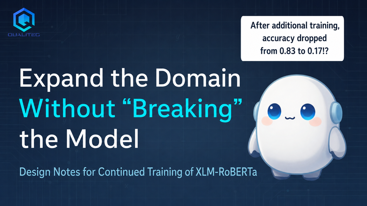
Precision tumbling from 0.83 all the way down to 0.17 — that really does happen.

In PII detection, the PII types to detect and the accuracy required can differ by domain. So even for a single engine, each time you extend coverage to a new domain, additional training (to adapt to that domain) may be required.

This article is an unvarnished account of the walls we hit in that effort to "extend domains through additional training," and the principles and judgments we took away from it.

This time, building on a fast Japanese NER model that uses XLM-RoBERTa as the encoder, we will write things down carefully in causal form: "because the method has this property, we designed it this way."

To give away the conclusion up front: the crux was not clever tricks for raising accuracy, but designing "what not to move."

We hope this proves useful to anyone standing in a similar spot.

0. Notation and the Model Foundation

We formulate NER as token classification. For an input sequence \(x=(x_1,\dots,x_T)\), an encoder \(f_\theta\) produces a contextual representation for each token, \(h_t = f_\theta(x)_t \in \mathbb{R}^d\), and a linear classification head \(W \in \mathbb{R}^{C\times d}\) (\(C\) is the number of labels, \(b\in\mathbb{R}^C\) is the bias) returns

$$ p(y_t = c \mid x) = \mathrm{softmax}(W h_t + b)_c = \frac{\exp(w_c^\top h_t + b_c)}{\sum_{c'} \exp(w_{c'}^\top h_t + b_{c'})} $$

. Training minimizes the cross-entropy \(\mathcal{L}=-\sum_t \log p(y_t^\star\mid x)\).

For the encoder \(f_\theta\) we use XLM-RoBERTa (multilingual RoBERTa).

Assume we already have, trained thoroughly on top of this \(f_\theta\), a

strong Japanese NER model \(M_0=(\theta_0, W_0)\)

. The goal is to extend coverage to new domains and new labels while preserving \(M_0\)'s strengths — in particular, its calibration of "not over-extracting from real-world prose."

Here, the degrees of freedom in additional training boil down to which parts of \(\theta\) (the encoder) and \(W\) (the head) to move, and by how much.

This entire article is about "how to constrain those degrees of freedom."

1. First, Understand XLM-RoBERTa's Properties (the Design Follows from Here)

Every design decision below derives from the following properties of XLM-RoBERTa.

(a) Multilingual, large-scale pretraining
XLM-RoBERTa is an encoder-only model pretrained with masked language modeling on a large corpus spanning roughly 100 languages. In general, lower layers carry cross-lingual, general-purpose features (morphology, grammar)、upper layers carry more task-oriented features — a layered structure that is empirically well known.
→ That is why, even when adding new capabilities, we adopted the policy of moving the lower layers as little as possible (the freezing, LoRA, and low learning rates described later). This is a design hypothesis based on general findings about layer-wise representations and on our own layer-wise freezing experiments — we are not asserting that calibration necessarily resides in the lower layers.

(b) SentencePiece subword tokenizer (Japanese has no whitespace boundaries)
A single word can split into multiple subwords, and entity boundaries can fall in the middle of a subword.
→ So we used character offsets (offset mapping) to align character spans with subwords, and assigned labels following the base model's tagging scheme. Note, however, that offset mapping only gives you the alignment — it does not resolve cases where a boundary falls inside a single subword. For such tokens you must choose a policy: "label if there is any overlap," "label only if fully contained," "use ignore_index," and so on. (If the base uses a single-tag scheme — no B/I prefixes — keep the single-tag scheme. Introducing B/I on your own splits the label space and muddies training.)

(c) Shared multilingual vocabulary
Romanized text, full-width/half-width variants, symbol-laden strings, and alphanumeric coinages can all be handled by splitting into subwords.
→ Hence even "proper names found in no dictionary and matched by no regex" — coinages that look like English words — can potentially be handled as contextual representations (though "can be split" and "robust to orthographic variation" are different things; we treat this as a hypothesis). This becomes the premise for the winning move described later: "going after new entity types through training."

(d) Encoder-only, plus a linear head
We assume that most of the task knowledge lives on the encoder side \(f_\theta\); the head \(W\) is merely a thin linear map. Moreover, \(f_\theta\) is shared across all domains and all labels.
→ Hence the trade-off discussed later — "a single encoder struggles to fully reconcile multiple domains" — arises. Move \(f_\theta\), and every decision riding on top of it moves too.

2. You Cannot Train What You Cannot Measure (Auditing the Evaluation)

Our first task was not new training but an audit of the evaluation metrics.

If the metric is off even slightly, every subsequent optimization heads in the wrong direction.
(Precision/Recall in this article are computed with overlap plus type match and micro averaging, excluding placeholders (markers of prior anonymization), comparing the bare model with no post-processing on the same held-out evaluation set. This is not exact match.)

In our case, the evaluation code turned out to have two main kinds of problems.

• Counting "markers that should not be detected" in Recall's denominator
  For example, if spans that were already redacted or symbolized in the source text are counted as "gold," the denominator in the definition of Recall
  $$ \text{Recall} = \frac{|\text{detected gold entities}|}{|\text{gold set}|} $$
  inflates and diverges from reality.
  What the product truly needs to protect are "entities whose leakage would hurt," so markers of prior anonymization should be excluded from the denominator.
  
• Gaps in the label mapping table
  If some conversions between the model's label names and the evaluator's expected names are missing, misses get overcounted for specific types only.

Fixing just these two issues changed the metrics substantially, and our understanding of the mission flipped: the weakness was not Recall but Precision (over-detection).

Lesson: measure-first. Before asking "why are the numbers bad," ask "is the definition of the numbers correct?" A bug in the metric becomes a source of major rework later.

3. Naive Continual Learning Causes "Forgetting" and "Skewed Training Distribution" at the Same Time

If you naively train only on the new domain's data (much of it synthetic), \(\theta_0 \to \theta\) shifts and performance on the old domains can drop. This can manifest as catastrophic forgetting — losing previously learned abilities through new training. However, the Precision collapse we observed cannot be explained by that alone (next paragraph).

What happens especially in NER is forgetting how to "stay silent on plain prose."

Synthetic sentences built from templates contain proper names in nearly every sentence. As a result, the prior probability (base rate) that a token is some entity

$$ \pi = \Pr(y_t \neq O) $$

becomes far higher in the training data than in real-world text. The model internalizes this skewed \(\pi\) and starts grabbing everything even in real prose.

In our observations, Precision fell to \(P\approx0.83\to0.17\) (Recall stayed high). Rather than catastrophic forgetting, this is the result of the model adapting to the distribution gap between synthetic data and real prose (shifted class priors and a shortage of negatives). In our case, both forgetting of old abilities and the skewed training distribution were involved.

Given XLM-RoBERTa's property (a), within the scope of our layer-wise freezing experiments the lower-layer representations were relatively well preserved, and what changed was most likely the calibration of the upper layers and the head (we did not rigorously identify this with layer-wise probes).
→ We therefore corrected the skew in \(\pi\) with two measures:

(1) bringing the synthetic data's density closer to real prose (placing proper names sparsely in long stretches of plain text so that \(O\) tokens dominate),

(2) hard negatives (sentences containing only common nouns or boilerplate, and confusable generic words).

Accuracy recovered, but within the frame of naive continued training it plateaued at a ceiling. The following sections are about breaking through it.

4. Do Not Rebuild the Classification Head (Decoy Classes as a Catch Basin)

The single most effective move was inheriting \(M_0\)'s label inventory as is.

This can be explained from two angles: how softmax probabilities behave, and the training signal.

Suppose you want \(k\) types (say person, organization, location), and you discard \(W_0\in\mathbb{R}^{C\times d}\) (\(C>k\)) to initialize a fresh \(W_{\text{new}}\in\mathbb{R}^{k\times d}\). Then the output slots that \(M_0\) held as separate classes — "product name," "facility," "event," and so on — the slots for non-target entities disappear。

Since softmax keeps probabilities summing to 1, the probability mass that sat on the removed classes gets redistributed to the remaining classes

$$ \text{remove class } C{+}1 \;\Rightarrow\; \text{renormalize to } \sum_{c=1}^{C} p(c\mid x)=1 \;\Rightarrow\; \arg\max_c \text{ can shift to a target type} $$

XLM-RoBERTa's encoder still represents the features saying "this word is a statute name / a facility name" — but there is no output slot left to receive them.

If you think of it as removing part of the existing logits, then losing the competing non-target classes makes the target classes more likely to be chosen. In practice, though, re-initializing the head changes the logits themselves, so you cannot strictly trace "mass that used to sit on that class leaked over." During retraining, the loss of existing decision boundaries, the absence of supervision for non-targets, and adaptation to the new data's class priors all contribute on top of this, leading to over-detection.

→ We therefore loaded \(W_0\) as is (matching the head shape on load, effectively ignore_mismatched_sizes=False), and designed training to give supervision only to the target-type labels

$$ \mathcal{L} = -\!\!\sum_{t:\, y_t^\star \in \{\text{target types}\}\cup\{O\}}\!\!\! \log p(y_t^\star \mid x) $$

By keeping the non-target "decoy" class rows as a warm start, \(M_0\)'s judgment that "this is not an organization but some other category" is less likely to be lost than with a freshly initialized head. (Whether it is strictly "preserved" is another matter — if the new data teaches non-targets uniformly as \(O\), negative gradients flow into the decoy rows as well. Ideally you protect the catch basin by pseudo-labeling old classes with a teacher model, using ignore_index for unannotated parts, adding replay, and so on.)This change alone visibly lifted the plateau.

Lesson: non-target classes have value as a "catch basin". Narrowing the types and rebuilding the head loses both the catch basin and the existing decision boundaries, increasing over-detection (softmax redistribution is one contributing factor).

5. Suppressing Drift with Self-Distillation (an Anchor That Resists Departure from the Base)

Even with decoys preserved, we could not reach \(M_0\)'s accuracy. Even light additional training drifts \(\theta\) bit by bit.

What works here is self-distillation.

The idea is this.

Instead of human annotation or dictionaries, teacher labels are created by having \(M_0\) itself run inference on real-world text, and the student (the model in training) is pulled toward the teacher's distribution

$$ \mathcal{L}_{\text{distill}} = \sum_t \mathrm{KL}\!\big(p_{M_0}(\cdot\mid x)\,\big\|\,p_{\theta}(\cdot\mid x)\big) $$

(Self-distillation in this article uses the same label space as \(M_0\) (teacher = student). Adding new types is a separate step in §6, done not with soft KL but with hard-label cross-entropy (the new type simply gets a label id), so there is never a point where KL is computed directly between teacher and student of different dimensions. Note that cross-entropy on hard-labeled \(M_0\) outputs is not the same as soft KL distillation — the probability information on non-argmax classes (dark knowledge) is lost.)

Ideally, this objective has \(p_\theta = p_{M_0}\) on the anchor data as its minimum. In practice, we train on finite anchor data, combine it with the new-type loss, and incur optimization error, so there is no guarantee of exact agreement with \(M_0\) on unseen data. Even so, in practical terms it works as a regularizer that strongly suppresses drift from additional training. With it, we were able to reproduce performance close to \(M_0\) on an independent old-domain evaluation set (separate from the anchors used for distillation). It is an effective move for avoiding "additional training = instant degradation."

A caveat is in order, though. Since the teacher is \(M_0\) itself, \(M_0\)'s quirks (such as over-detection) are easily inherited along with everything else on the anchor data.

That said, this does not mean "the student can never surpass the teacher." There are reports of students beating teachers even in same-architecture self-distillation, and adding new information from outside leaves room for improvement.

Self-distillation is therefore strictly a means of keeping existing behavior anchored to the base. To add a capability \(M_0\) does not have — such as a new type — you must bring in information from outside \(M_0\). That is the next section.

6. We Could Not Beat the Existing Domains — the Only Win Was "New Types Absent from the Output Space" (Head Surgery)

In theory, even on existing labels there is room to surpass \(M_0\) through higher-quality data, label-error correction, domain adaptation, better loss design, and so on (there are also reports of students beating teachers via self-distillation).
But with our data and methods, we never once exceeded the accuracy of the already-strong existing domains. We tried all five families touched on in §7 and confirmed in the production pipeline: every variant fell at or below the base. That is an honest negative result.
On the other hand, there was exactly one axis where we clearly won: new types that do not exist in \(M_0\)'s output label space. The existing model has no means of emitting those types at all, so this is a clear winning lane you can capture through training.

The typical case is a new entity type found in no dictionary and matched by no regex.

For example, proper names that are alphanumeric coinages slip past the dictionaries and regex rules we had prepared, and if \(M_0\) lacks the label, Recall is structurally \(0\). But as noted in §1(c), XLM-RoBERTa's multilingual subword representations leave room to treat such tokens contextually, and given an output slot, training can go capture them.

This is where learning-based NER can particularly shine.

The way to add it is head surgery: keep \(M_0\)'s classification layer \(W_0\in\mathbb{R}^{C\times d}\) intact and graft on one additional row for the new type

$$ W' = \begin{bmatrix} W_0 \\ w_{\text{new}}^\top \end{bmatrix} \in \mathbb{R}^{(C+1)\times d}, \qquad w_{\text{new}} \sim \mathcal{N}(0,\sigma^2 I),\ \ \sigma\!=\!0.02 $$

The existing \(C\) rows are reused as is (a warm start that carries over the existing logits), and one row is added for the new type. The new row is initialized as \(w_{\text{new}}\sim\mathcal{N}(0,\sigma^2 I)\), but since the variance of the new logit \(z_{\text{new}} = w_{\text{new}}^\top h + b\) is \(\sigma^2\|h\|^2\), a small \(\sigma\) does not keep the logit near 0 if \(\|h\|\) is large (for \(d=768\), the standard deviation is roughly \(0.02\sqrt{768}\approx 0.55\)). In other words, a small \(\sigma\) only zeroes the expectation; it is no guarantee the new class will not misfire. If you need to reliably suppress early misfires, place the new row's bias sufficiently negative and calibrate it on anchor data to the new-class false-positive rate you can tolerate. Also, "one added row" suffices only for a single-tag scheme; a BIO scheme requires multiple B-/I- rows.

old = model.classifier                  # Linear(d, C)
new = nn.Linear(d, C + 1)
with torch.no_grad():
    new.weight.normal_(std=0.02); new.bias.zero_()
    new.weight[:C] = old.weight         # copy existing rows (warm start)
    new.bias[:C]   = old.bias
model.classifier = new                  # train, focusing on the added row

* Because the code above replaces the entire classifier, as written both the existing \(C\) rows and the new row all become trainable. If you want to update only the new row, you must either mask the gradients of the old rows or implement old and new rows as separate Parameters. Note that PEFT's modules_to_save=["classifier"] does not merely "save" — it makes the whole classifier trainable.

With this method, we took the new type's Recall — which was \(0\) for \(M_0\) — and
recovered it to a practical level.

A number the base could never produce — and only here could we truly say we had "extended" the model.

7. LoRA: Deriving "Our Design" from First Principles

However, when we added the new capability, the shared encoder \(f_\theta\) moved, as §1(d) predicts, and in our experiments we ran into the problem of a slight accuracy drop in the existing domains.

The standard tool for minimizing this is the familiar LoRA (Low-Rank Adaptation).

Let us derive our decisions step by step from the principle.

7-1. The principle

LoRA rests on the hypothesis that the weight update \(\Delta W\) needed for fine-tuning can be approximated well by low-rank matrices (it has not been proven that "updates are inherently low-rank"; the hypothesis is that they have low intrinsic rank).

So instead of learning \(\Delta W\) in full, we express it as a low-rank decomposition,

$$ W = W_0 + \Delta W,\qquad \Delta W = \frac{\alpha}{r} BA,\quad B\in\mathbb{R}^{d\times r},\ A\in\mathbb{R}^{r\times k},\ r\ll \min(d,k) $$

Only \(A,B\) are trained, and the original \(W_0\) is fully frozen. \(\alpha\) is a scaling coefficient that adjusts the effective update magnitude via \(\alpha/r\).
(On notation: \(W_0\) here refers to a generic linear layer into which LoRA is inserted, distinct from the classification head \(W\) of §0.)

Two properties follow from this:

• It does not overwrite the base weights
  \(W_0\) is frozen and only \(A,B\) are trained. Because the rank of the update matrix \(\Delta W = BA\) is capped at \(r\), forgetting tends to be easier to suppress than with full fine-tuning — but "forgetting is always smaller" is not guaranteed, and the trade-off shifts with the task and the amount of training.
• Rank tends to act as a lever between plasticity and forgetting
  In our experiments, raising \(r\) strengthened adaptation to the new type but also tended to increase drift in the existing domains (though this also depends on the \(\alpha\) scaling, target layers, learning rate, and data distribution).

7-2. So this is how we reasoned

Our goal was

「to keep the existing domains behaving exactly like \(M_0\) while adding only the new entity type」

, so in light of LoRA's principle we designed as follows.

1. Freeze the base with LoRA
   The existing domains' calibration lives in \(W_0\) and \(f_{\theta_0}\), so not overwriting them is itself directly aligned with the goal.
   
   
2. Apply adaptation to the attention query / value
   In this configuration we restricted it to target_modules=["query","value"]. This choice follows the rule of thumb that adapting the attention mechanism works well; we are not claiming it is optimal for every NER task.
3. Keep the rank small (\(r=16\), \(\alpha=32\))
   Adding a single new type does not require much expressive power, so we prioritized suppressing forgetting.
   Indeed, raising \(r\) caused the existing domains to drift.
   
   
4. Treat the head separately
   The new-type row needs training, so the classification head stays trainable as an exception to the LoRA freeze (modules_to_save=["classifier"]).
   Going a step further, we also tried a variant that freezes only the existing label rows via gradient masking and trains only the new-type row. (Note that even with gradients stopped, weight decay applied to the classifier can still move the existing rows, so you need precautions such as setting the classifier's weight decay to 0.)
5. Raise the learning rate for LoRA
   Standard LoRA zero-initializes \(B\), so right after insertion the update starts from zero (a no-op). The newly added adapter and the new head row must adapt in a short time, and our validation showed that the tiny \(\text{lr}=5\times10^{-6}\) used for head preservation and self-distillation was not enough — \(\text{lr}=2\times10^{-4}\) for 2 epochs was what worked.
   The point to watch: it is not "we froze most things, so apply it gently."
6. Merge after training
   At inference time, fold in \(W=W_0+\frac{\alpha}{r}BA\) (merge_and_unload), and save it as ordinary weights。
   Consumers just swap the file in; they never need to know LoRA was involved.
   
   

7-3. The "Shared-Encoder Reconciliation Cost" That Remains Regardless

This is the essential finding.

Even with \(W_0\) and the existing head rows frozen, LoRA moves the shared encoder's internal representations, so the existing domains' logits in general carry no guarantee of matching the original model。

$$ \underbrace{W_0\, f_{\theta_0+\Delta}(x)}_{\text{existing-head output after LoRA}} \;\not\equiv\; \underbrace{W_0\, f_{\theta_0}(x)}_{\text{output of } M_0} $$

As long as \(f\) is shared across all domains, inserting \(\Delta\) for the new type means that \(\Delta\) can also move the existing domains' \(h_t\). We tried five families — "full mixed training," "lower-layer freezing," "LoRA," "LoRA plus frozen existing head," and "data-mix changes" — and the existing domains' accuracy stuck to nearly the same ceiling in every one.

We also confirmed a side effect: freeze the lower layers too aggressively and the new type can no longer be learned — Recall collapses to \(0\) (plasticity is lost).

Conclusion: among the five configurations we tried, none fully preserved the existing domains while adequately acquiring the new type. Our interpretation is that updates to the shared encoder's representations act as interference against the existing domains (in principle, room remains to reconcile the two with replay, functional regularization, conditional routing, and the like). Full separation would mean a different architecture — per-domain adapters or split models — to be weighed against the operational constraint of wanting a single integrated engine.

8. Crush Leakage Using "the Domain's Document Structure"

In additional training, if evaluation data seeps into training, the numbers become lies.

Excluding the evaluation set by ID goes without saying, but in domains where documents quote each other at length (court rulings, academic papers, and the like), that alone is insufficient.
A training document with a different ID can contain dozens of characters of an evaluation document's body verbatim.

→ So we chopped each evaluation document into windows (shingles) of length \(k\) and matched them against the training side by partial match,

$$ \text{leak}(d_{\text{train}}) = \mathbb{1}\!\Big[\,\exists\, s \in \mathrm{Shingles}_k(\mathcal{E}):\ s \subseteq d_{\text{train}}\,\Big],\qquad k=50 $$

(\(\mathcal{E}\) is the full text of the evaluation set.)
Partial matches that naive spot-check probing would miss are, with shingle matching, caught with high accuracy for long exact matches (though normalization differences, OCR errors, paraphrases, and overlaps of 49 characters or fewer still slip through).
When in doubt we err toward exclusion, but long matches on boilerplate can over-exclude and distort the distribution, so we keep an eye on the counts.

Lesson: design your leakage defenses around the domain's document structure (quotation, boilerplate). ID-match checks alone are not enough.

9. In the End, Decide by "the Asymmetry of Costs"

When accuracy metrics are contested at the decimal level, the final call should be made not by which number is larger but by the asymmetry of error costs.

In many real-world tasks, the costs of a miss (FN) and an over-detection (FP) differ greatly

$$ \text{cost} = \lambda_{\text{FN}}\cdot \mathrm{FN} + \lambda_{\text{FP}}\cdot \mathrm{FP},\qquad \lambda_{\text{FN}} \gg \lambda_{\text{FP}} $$

If misses are fatal for your task, then a model that keeps Recall while giving up a sliver of Precision (i.e., leans toward the over-detecting side) is worth adopting, provided it recovers substantial misses in another domain.

In fact, the version we moved to adoption traded a very slight drop in existing-domain Precision for maintained Recall (no additional misses on the evaluation set) while recovering a large share of the new type's misses.

That said, this weighting — where to draw the lower gate on precision — is a product value judgment, and the model side should not decide it unilaterally.

The right path is to hand the field numbers to the decision-makers — the product manager and peers.

10. Practical Tips (Small Things That Worked — or Turned Out to Be Traps)

Here we share implementation-level findings that quietly mattered (or bit us) behind the principles.

Training recipe

• The stronger the base, the lighter the touch
  With this model and data mix, head preservation plus self-distillation needed only \(\text{lr}=5\times10^{-6}\) and 1 epoch. Push harder and it tips straight into over-detection.
• LoRA, conversely, needs a firmer touch
  Standard LoRA starts from a \(B\)-zero initialization (an initial no-op), and the new adapter and new head row must adapt quickly, so this configuration needed around \(\text{lr}=2\times10^{-4}\) and 2 epochs.
• Freeze too much and the new type cannot be learned
  When we froze the lower layers thickly, the existing domains stayed untouched but the new type's Recall collapsed to \(0\). Keep some plasticity.
  
  

Labels and the head

• Match the base's tagging scheme (single-tag if the base is single-tag).
  Adding B/I on your own splits the label space.
  
  
• Oversample the new type
  Its occurrences are few, so duplicate them severalfold within the training set. Generating values that change every time reduces the risk of memorizing the literal strings (though template structure and surrounding context can still be memorized, so it is not fully "safe" — and note that oversampling also shifts the class priors).
• Merge and ship a "plain model"
  Consumers just swap the file. Keep output label names aligned with the base so the new type can be absorbed with a one-line mapping addition on the consumer side.
  

Synthetic data design (teaching the model to "stay silent")

• density
  Stop doing one entity per sentence; scatter proper names sparsely through plain prose.
  
  
• Contrastive minimal pairs
  Show pairs with identical sentence frames — "with proper-name modifier = target type" versus "bare generic noun / demonstrative + generic noun = \(O\)" — so the model generalizes that "the presence of the modifier decides the type."
  
  
• Generic terms, boilerplate, redactions, and fragments are \(O\)
  For example, for the ADDRESS PII type, a teacher signal that "trims down to the administrative-district prefix and keeps that" can also be effective.
  
  

Use real-world text as clean negatives

• From public real-world text, take sentences that match no known proper-noun dictionary as negative candidates (with dictionary matching accelerated by Aho-Corasick), then run them through teacher-model agreement, multiple detectors, and sampling audits before using them as all-\(O\) silver negatives. "Not in the dictionary" does not mean "no entity present" (indeed, the very "new proper names outside dictionaries" this article targets can become false negatives), so avoid blanket, machine-decided all-\(O\) labeling.
• Floods of near-identical sentences (templates differing only in the year, etc.) are suppressed with deduplication on signatures with numerals folded away.

Evaluation traps

• A same-distribution synthetic dev set tends to be optimistic
  Because templates and generation rules overlap with the training set, numbers skew optimistic. Treat it as a guide for early stopping, no more.
• Rising Recall alone does not imply over-detection(FPs do not enter Recall.) But if a Recall rise coincides with a Precision plunge, a surge in predicted span counts, or concentration on particular labels, suspect over-detection. Always read Recall and Precision together.
• Local metrics may not proxy the production pipeline. With downstream sieves (dictionaries, deny lists), bare-model Precision and production Precision do not correspond linearly.Finalize the data mix ratio using feedback from production evaluation。

Schema and operations

• Variation in the label keys from upstream (label / entity_type) should be accepted on both forms at the ingestion point.
  
  
• Bulk label renames (versioning the label inventory) should be machine-converted, and applied only after confirming that "base metrics are unchanged after conversion," proving the rename is pure.
  
  
• The minimal guard against new-type misfires (single-character false detections and the like) belongs, without distorting the model, in thin post-processing on the consumer side.

The Art of Extending Comes Down to Designing What Not to Move

Let us recap the lessons on extending (domains) that we have covered.

1. measure-first
   Crush evaluation-definition bugs first
   (the handling of anonymization and label conversion can transform the metrics).
   
2. Respect XLM-RoBERTa's layered structure
   Treat "protect the lower layers" as a design hypothesis and validate it with layer-wise freezing experiments.
3. Do not casually rebuild the head
   Do not casually discard the existing decision boundaries and the output slots for non-target classes.
4. Anchor with self-distillation
   Teacher = yourself, as a regularizer that suppresses drift. Adding new capability requires outside information.
5. One clear avenue for extension is new types
   For types absent from the existing label space, extend the head and add a trainable output slot.
6. Design LoRA from first principles
   Translate the tendency of low-rank updates to suppress forgetting into concrete choices: freezing, low rank, and separate head handling. (Even then, the shared-encoder reconciliation cost remains.)
7. Leakage by structure; decisions by asymmetric cost。

Closing

So there it is: a full tour of the design philosophy for extending an XLM-RoBERTa-based NER model "without breaking it" — starting with the evaluation audit, then decoy-class preservation, self-distillation anchoring, head surgery, LoRA, and finally leakage defenses and cost asymmetry.

The through-line was, consistently, the idea of "designing what not to move."

Additional training is a tightrope walk where moving the base even slightly risks degradation.

That is precisely why the real work was not accuracy tricks but discerning "what to freeze, and what alone to move."

If you are looking to evolve a model you have already built — wisely — we hope something here serves as a hint.

Next time, we plan to bring you more hands-on, down-to-earth findings from the machine learning field.

Thank you very much for reading to the end.