AI Mathematics

How to Build AI Lipsync, Part 3: Learning to Map wav2vec Features to Mouth-Shape Parameters

Qualiteg Research Team

Jul 14, 2025 — 12 min read

Hello!

In the previous installments of this series, we covered

. This time, we finally step into the heart of the matter: integrating these techniques to actually generate mouth movements from speech.

This article covers the training process that converts the 768-dimensional acoustic features extracted by wav2vec into time-series data for 26 mouth-shape control parameters. This is not mere dimensionality reduction. It is a conversion from a high-dimensional vector representing the physical properties of sound into an entirely different modality: human mouth movement. To achieve this conversion, a neural network must learn the complex correspondence between phonemes and visible mouth shapes.

What makes this especially challenging is that the correspondence is dynamic, not static. The same phoneme takes different mouth shapes depending on the surrounding context, and there is also a temporal offset: the mouth begins moving before the sound is even heard. How do we model and train for such complex phenomena? In this article, we compare two powerful approaches — LSTMs and Transformers — and search for the best method from a practical standpoint.

1. The Essence of the Problem: Why Mouth-Shape Prediction Is Hard

1.1 The Same Phoneme, Different Mouth Shapes Depending on Context

To understand why lipsync is difficult, let's start with the Japanese phoneme ん ("n") as an example. Any Japanese speaker can pronounce this sound, yet the mouth shape actually varies substantially with the situation.

When you say さんぽ (sanpo, "a walk"), the lips already begin to close during the ん. That is because the following ぽ (po) is a bilabial plosive, which requires the lips to close completely. In contrast, for the ん in さんか (sanka, "participation"), the lips do not close. The following か (ka) is a velar plosive, articulated at the back of the mouth, so there is no need to close the lips.

This phenomenon is called coarticulation and is observed universally in natural human speech. Our brains unconsciously predict the upcoming sound and plan efficient mouth movements accordingly.

This predictive movement is precisely the key to achieving natural lipsync.

1.2 Mouth Movements That Precede the Audio

Even more interesting is the phenomenon of mouth movement preceding the actual sound. When human speech is filmed with a high-speed camera, the mouth can be seen starting to move 50 to 100 milliseconds before the sound is heard.

Plosives are the most striking example. When you produce the sound ぱ (pa), you first close your lips to build up pressure in the oral cavity, then release them to create the plosive. In other words, by the moment the sound is heard, the lips have already begun to open. If this temporal offset is not modeled accurately, the audio and the mouth movement appear out of sync, resulting in unnatural lipsync.

1.3 The Complex Phenomenon of Coarticulation

Coarticulation is not limited to the influence between adjacent phonemes; it extends over a much wider range. Consider, for example, the utterance ありがとうございます (arigatou gozaimasu, "thank you").

From this installment on, the mechanisms we discuss get a bit more involved, so we are bringing in "Professor Quo" and his student "Manabu" — their conversations will help us deepen our understanding!

Prof. Quo: Now, let's think about the mouth shape when pronouncing the が (ga) in ありがとうございます (arigatou gozaimasu, "thank you"). Is there any difference from saying が on its own?

Manabu: Professor, before that — this is your first appearance today, so please introduce yourself!

Prof. Quo: I am Professor Quo, pleased to meet you. My hobby is explaining tricky AI topics with simple analogies. Now, back to where we were. Let's think about the mouth shape when pronouncing the が in ありがとうございます. Is there any difference from saying が normally?

Manabu: Hmm, I don't really notice any difference...

Prof. Quo: Try pronouncing it slowly while looking in a mirror. First say が on its own, then the が inside ありがとう (arigatou).

Manabu: Oh! It really is different. With the が in ありがとう, my mouth doesn't open as much...

Prof. Quo: Excellent observation! Because of the preceding り (ri), the tongue is still positioned high in the mouth — and, even more interestingly, preparation for the following とう (tou) has already begun.

Manabu: What? Already preparing for とう at the moment of が?

Prof. Quo: That's right. The う (u) in とう is a sound that rounds the lips. If you look closely, the mouth is already beginning to round slightly at the が. In other words, the mouth is being influenced by a sound as far as three steps ahead.

Manabu: Amazing! The human brain really does compute that far ahead.

Prof. Quo: Exactly. That's why, when building lipsync on a computer, a simple lookup table of "this sound maps to this mouth shape" is not enough. You need to take a wide range of surrounding sounds into account.

To handle such complex phenomena, we need sophisticated machine learning models. In the next chapter, we take a detailed look at the first approach to this challenge: time-series modeling with LSTMs.

2. Time-Series Modeling with LSTMs

2.1 Why a Simple Neural Network Won't Do

The first approach that comes to mind might be a simple fully connected neural network that takes the wav2vec features at each time step as input and outputs the corresponding mouth-shape parameters. This approach, however, has a fatal flaw.

A simple neural network processes each time step independently and therefore cannot take temporal context into account at all. In the さんぽ (sanpo) example above, at the ん it cannot use the information that "ぽ comes next." As a result, it outputs the same mouth shape for every ん, producing extremely unnatural lipsync.

Prof. Quo: Let me explain the problem with simple neural networks using a more familiar example. Think about weather forecasting.

Manabu: Weather forecasting?

Prof. Quo: Yes. What if you tried to forecast tomorrow's weather from today's temperature alone?

Manabu: That would be tough. You would also need past information — how things have changed since yesterday, how the atmospheric pressure is moving, and so on.

Prof. Quo: Exactly! Lipsync is the same. To decide the mouth shape for the sound ん (n), you need context — what sounds came before it and what sounds come after it. But a simple neural network only sees the information at this very moment.

Manabu: I see — so that's why it ends up looking unnatural.

2.2 The Basic Idea of RNNs and Their Limitations

RNNs (Recurrent Neural Networks) emerged to solve this problem. An RNN is a neural network with "memory": it can process time-series data while retaining information about the past.

The basic idea of an RNN is to compute the current output using not only the current input but also the internal state from the previous time step. This makes predictions that take past context into account possible.

However, RNNs suffer from a serious issue known as the "vanishing gradient problem." As the sequence grows longer, the influence of past information decays exponentially.

Prof. Quo: Let me explain the vanishing gradient problem in RNNs with the game of telephone.

Manabu: Another analogy! The telephone game, then.

Prof. Quo: Yes. Suppose ten people play the telephone game. If the first person says, "It's sunny and pleasant today," will that message reach the tenth person intact?

Manabu: Probably not. It changes little by little along the way, and by the end it would be something completely different.

Prof. Quo: Exactly. RNNs are the same — as information is passed from step to step, it fades more and more. Mathematically speaking, if it shrinks to 0.9x at each step, after 10 steps it is 0.9 to the 10th power, about 0.35x, and after 20 steps only about 0.12x remains.

Manabu: So the information from the beginning of a long sentence never makes it to the end.

Prof. Quo: That is precisely the problem. In a sentence like "The weather was nice today, so I went to the park, played with my friends, and ate ice cream," when you predict the mouth shape for the final "ate," almost none of the information from the opening "today" is left.

2.3 The "Memory" Problem LSTMs Solve

LSTM (Long Short-Term Memory) is a special kind of RNN designed to solve this vanishing gradient problem. The LSTM's key innovation is the introduction of "gate mechanisms" that control the flow of information.

Prof. Quo: Let me explain the LSTM's gate mechanism using how a library works.

Manabu: A library? Another fun analogy. I knew a little about RNNs, but LSTMs always seemed difficult — I never really understood them.

Prof. Quo: A library has three important functions. First, the "forget gate" is the librarian who disposes of outdated books. Books nobody reads anymore get discarded to free up space.

Manabu: I see — it throws away unneeded information. In memory terms, unnecessary memories simply get forgotten.

Prof. Quo: Next, the "input gate" is the librarian who selects and purchases new books. Not every book gets bought — only the important ones are added to the library.

Manabu: So it memorizes only the important information.

Prof. Quo: Exactly. Finally, the "output gate" is the librarian who finds and hands over the book a visitor is looking for. Rather than handing over every book in the library, they pick out only the books needed right now.

Manabu: In other words, it retrieves only the information that's needed.

Prof. Quo: Precisely! Using these three gates, an LSTM can store necessary information for long periods, forget what is unnecessary, and retrieve just the information it needs exactly when it needs it. That is why it is called "Long Short-Term Memory."

With these gate mechanisms, an LSTM can retain necessary information over long spans and appropriately forget what it no longer needs. In lipsync terms, it can hold on to information like "this utterance is a question" all the way to the end of the sentence, while forgetting the details of individual phonemes at the right time.

2.4 Why We Need Bidirectional LSTMs: Looking at Both Past and Future

A standard LSTM handles only the flow of information from the past to the present. In lipsync, however, future information matters too. The lips begin to close at the ん in さんぽ (sanpo) precisely because we know the ぽ is coming.

Bidirectional LSTMs solve this problem. They process the sequence in both the forward direction (past to future) and the backward direction (future to past), and integrate information from both directions at each time step.

Prof. Quo: Let me explain how bidirectional LSTMs work with a film-editing analogy.

Manabu: After the librarians, now film editing? Professor, you really do come up with all kinds of analogies.

Prof. Quo: Yes. When editing a film, to decide how to cut a given scene, you need to look at what comes before and after it, right?

Manabu: True. You have to consider the flow from the previous scene and the transition into the next one.

Prof. Quo: That is exactly what a bidirectional LSTM does. For example, in the utterance こんにちは (konnichiwa, "hello"), when deciding the mouth shape for に (ni), the forward LSTM holds the past information こん (kon) — it tells us, "we have said kon so far, so the mouth is in this state."

Manabu: I see. So if there's a forward one, what does the backward LSTM do?

Prof. Quo: The backward LSTM processes from the future toward the past, so it provides information like, "ちは (chiwa) comes next, so the mouth needs to prepare like this."

Manabu: With information from both directions — past to future and future to past — you can predict the mouth shape much more accurately!

Prof. Quo: Exactly. Humans actually do this unconsciously as well. Because we know what we are about to say, we can prepare our mouths in advance. You could say bidirectional LSTMs mimic this natural human speech mechanism.

With a bidirectional LSTM, mouth-shape prediction at each time step can take both past and future context into account. This is a crucial ingredient for achieving natural lipsync.

3. Designing an LSTM-Based Network

3.1 Overall Architecture (wav2vec to Mouth-Shape Parameters)

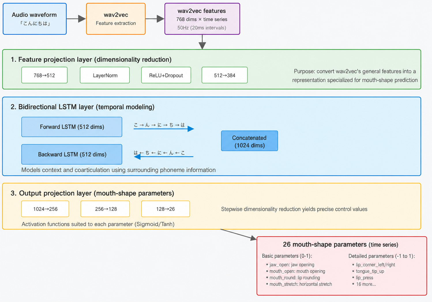
To get a visual understanding of the actual network structure, let's look at the architecture diagram above. It shows the entire conversion process from the audio waveform to the mouth-shape parameters, organized into three broad stages: input processing, the main network, and output generation.

3.2 The Role of Each Layer

Feature projection layer: reducing 768 dimensions to 384

The 768-dimensional features output by wav2vec contain every kind of information about the audio: speaker characteristics, emotion, environmental sounds, and the phonetic information we actually need, all mixed together. For lipsync, however, what matters is primarily the phonetic information and the related prosodic information.

The role of this layer is to extract only the information needed for mouth-shape prediction from the high-dimensional 768-dimensional space and compress it into a more manageable 384 dimensions. Beyond a simple linear transformation, it combines LayerNormalization for normalization, a ReLU activation for nonlinearity, and Dropout to prevent overfitting, achieving robust feature extraction.

Manabu: What was dimensionality reduction again? Could you explain it with another analogy?

Prof. Quo: Sure — let me explain dimensionality reduction with photo editing.

Manabu: Photo editing it is.

Prof. Quo: Yes. A photo taken with your smartphone contains a lot of information — not just the subject, but also the background, the lighting, the color temperature, and so on. But what if you want to crop out just a person's face?

Manabu: You remove the background and keep only the face.

Prof. Quo: Exactly! wav2vec's 768 dimensions are like a high-resolution photo holding "all the information about the sound." But for mouth-shape prediction, we only need the "face" — the phonetic information. So we strip out the unneeded background (speaker identity, environmental sounds, and so on) and compress just the necessary parts into 384 dimensions.

Manabu: I see! But isn't there a risk of compressing too much and losing important information?

Prof. Quo: Good question. That's why we compress in stages: reducing 768 → 512 → 384 in two steps prevents an abrupt loss of information. And by inserting LayerNorm and Dropout at each stage, we make sure the important information reliably reaches the next layer.

Bidirectional LSTM layers: learning temporal patterns

These layers are the heart of the network. The forward LSTM and the backward LSTM each maintain a 512-dimensional hidden state, together producing 1024 dimensions of contextual information.

The forward LSTM processes こ→ん→に→ち→は (ko → n → ni → chi → wa) in order, accumulating at each step the information of "what has been said so far." The backward LSTM processes the sequence in reverse, providing the information of "what will be said next." Integrating the two yields a representation at each time step that accounts for both past and future context.

Stacking three LSTM layers allows the network to learn more complex temporal patterns. You can think of the first layer as capturing basic phoneme transitions, the second layer coarticulation patterns, and the third layer longer-range dependencies.

Output projection layer: converting 384 dimensions to 26

The final output layer converts the 1024-dimensional contextual representation produced by the LSTM into the 26 mouth-shape parameters. Here too, the transformation proceeds in stages (1024 → 256 → 128 → 26) to avoid abrupt information compression.

Especially important is choosing activation functions to match the characteristics of each parameter. Parameters that range from 0 to 1, such as jaw_open and mouth_open, use a Sigmoid function, while parameters that range from -1 to 1, such as lip_corner_left, use a Tanh function.

3.3 Why This Architecture Works

The reason this network architecture is effective is that it mimics the human speech mechanism.

First, the feature projection layer corresponds to the human auditory system: the process of extracting only speech-related information from the sound entering the ears. Next, the bidirectional LSTM layers correspond to the brain's language-processing regions, integrating past context and future plans to generate appropriate motor commands. Finally, the output projection layer corresponds to the motor control system, converting abstract commands into concrete muscle movements.

Prof. Quo: Let's compare this whole network to an orchestra conductor.

Manabu: Why would a trained model be a conductor?

Prof. Quo: Well, a conductor reads the score (the wav2vec features) and turns it into instructions for the performers (the mouth-shape parameters), right? But they are not merely looking at the current measure.

Manabu: True — a conductor conducts the present moment with the flow of the whole piece in mind.

Prof. Quo: Exactly! The feature projection layer is the ability to read the important parts out of a complex score. The bidirectional LSTM is the ability to consider the past performance and the future development at the same time. And the output projection layer is the ability to turn all of that into concrete instructions for each instrumentalist (each mouth-shape parameter).

Manabu: I see! So that's why each layer has a clear role.

Prof. Quo: Precisely. And what matters is that these layers work in concert. If any one of them is missing, natural lipsync cannot be achieved. It's just like human speech, which becomes possible only when hearing, language processing, and motor control work together.

An LSTM network designed this way can learn efficiently even from limited data and generate natural lipsync.

Summary

In this article, we began exploring the core of lipsync technology: converting wav2vec features into mouth-shape parameters.

We got to the heart of why this problem is hard. Through the coarticulation example of the same sound ん taking different mouth shapes in さんぽ (sanpo) and さんか (sanka), we saw how much context matters. The phenomenon of the mouth starting to move 50 to 100 milliseconds ahead of the audio also speaks to the complexity of lipsync.

As a first approach to this time-series problem, we walked through LSTMs in detail. Through the dialogue between Professor Quo and Manabu, we learned how the LSTM's gate mechanisms (forget, input, and output gates) solve the RNN vanishing gradient problem. The ability of bidirectional LSTMs to consider both past and future context is especially important.

Finally, we introduced an example of an LSTM-based network: a projection layer that compresses the 768-dimensional wav2vec features to 384 dimensions, bidirectional LSTM layers that learn temporal patterns, and an output layer that generates the 26 mouth-shape parameters.

Next time, we will move on to the more practical topics of data preparation and the training process, and also look at the limitations of LSTMs and a newer approach: the Transformer.

See you in the next installment!