LLM

LLM Inference Infrastructure Provisioning Course, Part 2: Estimating Request Volume for an LLM Service

Qualiteg Consulting

May 29, 2025 — 8 min read

Hello!
Welcome to Part 2 of the LLM Inference Infrastructure Provisioning Course.

LLM Inference Infrastructure Provisioning Course: Series Index

STEP 2: Estimating Request Volume for an LLM Service

Let's dive right into the second step of LLM inference infrastructure provisioning: estimating request volume. We will look at why it matters and how to do it.

To properly estimate the number of GPU nodes required when building an LLM service, you first need an accurate prediction of the number of requests the service is expected to receive.

The Basic Approach to Request Estimation

Deriving the required number of GPU nodes from the expected request volume of your LLM service is a critical part of service design. Underestimate it and service quality suffers; overestimate it and you pay for capacity you never use. Request estimation is the foundation for striking the right balance.

Parameters for Estimating Expected Request Volume

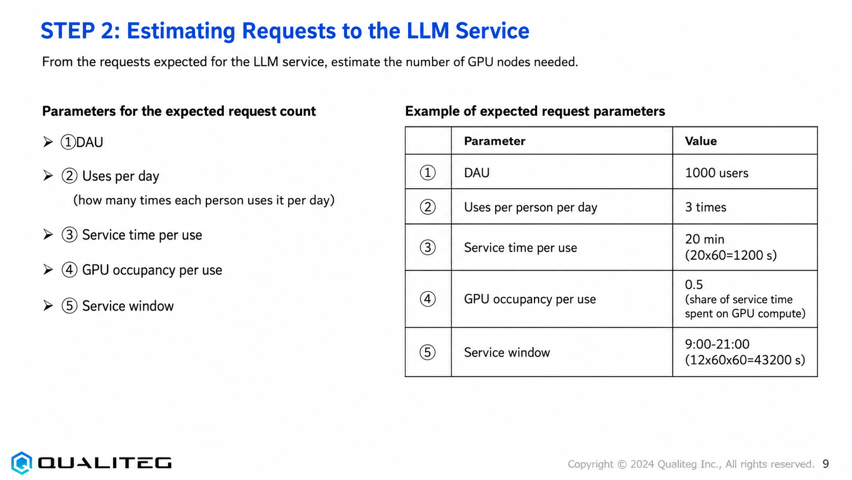
Let's look at the five key parameters used to estimate request volume.

DAU (Daily Active Users): The number of users who actually use the service in a day. This is the most fundamental indicator of a service's scale.
Uses per user per day: A frequency metric indicating how many times each user uses the service in a day. Total request volume varies significantly depending on this value.
Usage time per session: The average amount of time (in seconds) a user spends on the service in a single session. For LLM services, this corresponds to the time spent conversing with the model or generating content.
GPU occupancy rate per session: The fraction of session time actually spent on GPU computation. The GPU is not running at full tilt the whole time; this metric accounts for idle periods such as waiting for user input.
Service hours: The hours of the day during which the service is available. Some services run 24/7, while others are available only during business hours (e.g., 9:00 to 21:00).

A Concrete Example of Expected Request Volume

Working through concrete numbers makes all of this much clearer, so let's use the following figures.

DAU: 1,000 users — assuming a mid-sized enterprise LLM service
Uses per user per day: 3 — each user uses the service an average of three times a day
Usage time per session: 20 minutes (20 × 60 = 1,200 seconds) — the time spent conversing with the LLM or generating content
GPU occupancy rate per session: 0.5 (50%) — the fraction of session time actually spent on GPU computation
Service hours: 9:00 to 21:00 (12 hours = 12 × 60 × 60 = 43,200 seconds) — assuming business hours

In this example, the service is used a total of 3,000 times per day (1,000 users × 3 uses), each session takes 20 minutes on average, and roughly half of that time is spent on GPU computation. The service is available 12 hours a day.

The point is to work with realistic figures that reflect your use case — here, a domain-specific enterprise LLM service such as an internal knowledge-base search and question-answering system.

Deriving the Number of Concurrent Requests

Now, using the five parameters above, let's calculate the GPU resources the LLM service actually needs.

Here we will walk through the process in detail: first computing the total GPU time required from the expected request volume, then deriving the number of concurrent requests from it.

Calculating "Total GPU Time"

Total GPU time is the sum of all GPU processing time required to operate the LLM service. It represents the total GPU running time needed to handle every user request.

The formula is as follows.

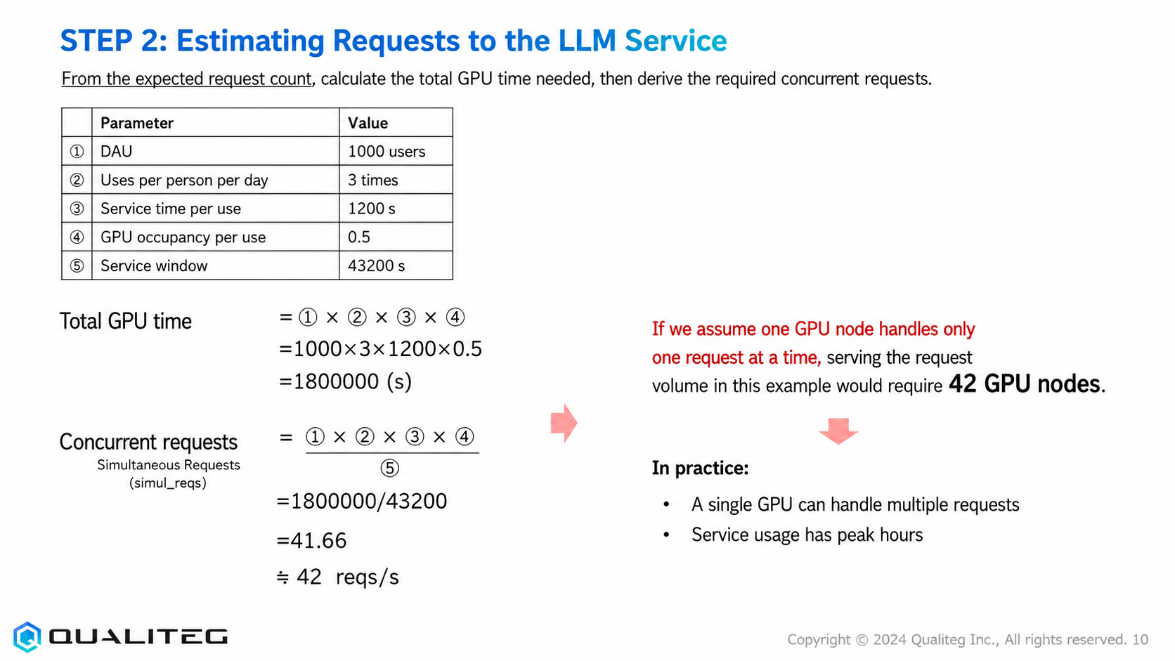
Total GPU time = ① DAU × ② Uses per user per day × ③ Usage time per session × ④ GPU occupancy rate

Plugging in the actual numbers:

DAU: 1,000 users
Uses per user per day: 3
Usage time per session: 1,200 seconds
GPU occupancy rate: 0.5

Total GPU time = 1,000 × 3 × 1,200 × 0.5 = 1,800,000 (seconds)

This result tells us that roughly 1,800,000 seconds (about 500 hours) of GPU processing time is required per day.

Calculating the "Number of Concurrent Requests"

The next important step is calculating the number of concurrent requests: the average number of requests that must be processed simultaneously during service hours. The formula is as follows.

Concurrent requests = (① DAU × ② Uses per user per day × ③ Usage time per session × ④ GPU occupancy rate) ÷ ⑤ Service hours

That is, concurrent requests = 1,800,000 ÷ 43,200 = 41.66 ≈ 42 reqs/s

In other words, this LLM service needs the capacity to handle an average of 42 concurrent requests per second.

Estimating the Number of GPU Nodes

So how many GPU nodes would it take to handle these requests?

To build intuition, let's start with a somewhat extreme simplification. If we assume that

"each GPU node handles only one request"

, then handling the request volume in our example works out to

"42 GPU nodes required."

That is what the arithmetic tells us.

Of course, this is the crudest possible estimate — one GPU per concurrent user is a rather blunt approach. So let's refine it by letting a single GPU serve multiple requests and by considering how access is distributed over time.

Sidebar
GPUs themselves are actually not designed for "concurrent access."
Only one user (a program, rather than a person) can access a GPU at a time.
That phrasing, however, can be misleading.
A GPU can perform an enormous number of computations at once — in parallel. But when multiple users access the service simultaneously over the internet, juggling those requests is not the GPU's job; it is the job of the software that manages the GPU. That software applies various techniques to transform requests from many users into what looks like "one giant computation" from the GPU's point of view. We won't go into detail in this article, but we also develop such technologies for distributing work efficiently across GPUs, known as "continuous batching" and "distributed batching": https://blog.qualiteg.com/deep_learning_model_safe_inference_and_pooling/

A Single GPU Handles Multiple Requests
In practice, a GPU can often process multiple requests simultaneously, depending on its memory capacity and the model size. If one GPU can handle, say, two to four requests at the same time, the number of GPUs required drops significantly.
Service Usage Has Peak Hours
Actual service usage is not uniform throughout the day; it typically concentrates in specific time slots. For a business-hours service, for instance, requests tend to cluster in particular mid-morning or afternoon periods. The system must be designed to handle this peak load.

Taking these two factors into account yields a more realistic estimate of the required GPU nodes. For example, if one GPU can process an average of three requests concurrently and peak traffic is 1.5 times the average:

Required GPU nodes = 42 ÷ 3 × 1.5 ≈ 21

This is how the calculation can be refined.

Accounting for Peak Request Hours in an LLM Service

In real-world service operations, there is a more practical factor we need to take into account: peak hours.

Let's look at how to estimate request volume at peak times.

Why Peak-Hour Request Volume Matters

When sizing a GPU-backed LLM service, what matters is not the average traffic but the request volume during peak hours — the period with the highest concurrency. A service's stability and quality are judged by how well it functions under peak load.

It is common for requests to concentrate in particular time slots during the day. For an in-house LLM service, for example, usage may spike during pre-meeting research, right after lunch, or in the evening when people wrap up their work. The system must be designed to deliver sufficient performance at these peaks.

A Peak-Hour Calculation Example

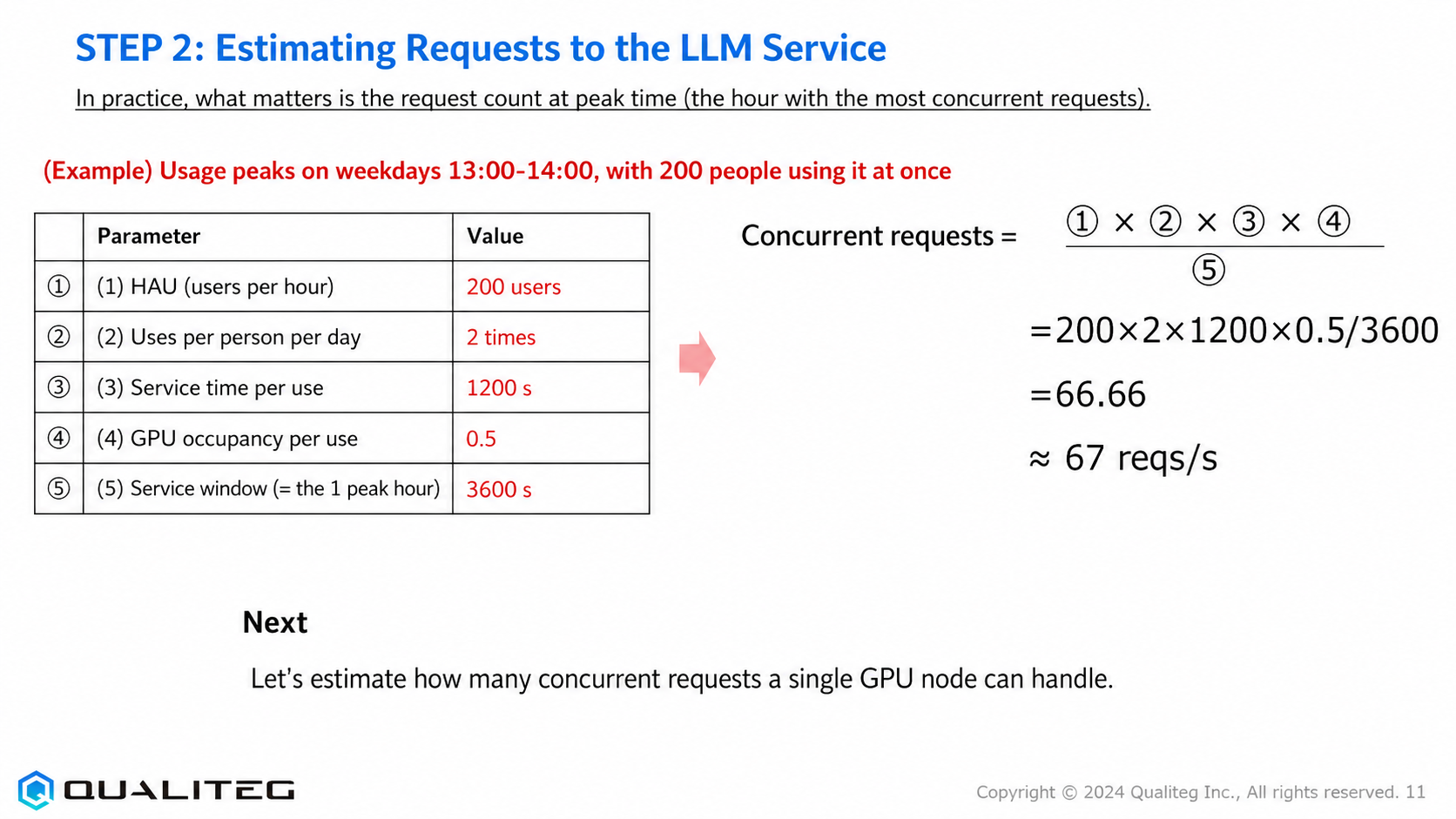
As a concrete example, the figure presents the scenario "usage peaks between 13:00 and 14:00 on weekdays, with 200 people using the service at once." The five parameters for this peak hour are set as follows.

HAU (users per hour): 200 users — the number of users concentrated in the peak hour
Uses per user per day: 2 — the average number of uses within the peak hour
Usage time per session: 1,200 seconds — the duration of a single session
GPU occupancy rate per session: 0.5 — the fraction of time the GPU is actually in use
Service hours (the one-hour peak window): 3,600 seconds — the time frame the calculation is based on

Using these values, let's calculate the number of concurrent requests at peak time.

Concurrent requests = (① HAU × ② Uses per user × ③ Usage time per session × ④ GPU occupancy rate) ÷ ⑤ Service hours

Substituting in the actual numbers:

Concurrent requests = (200 × 2 × 1200 × 0.5) ÷ 3600 = 66.66 ≈ 67 reqs/s

This result shows that during the peak hour the service needs the capacity to process roughly 67 concurrent requests per second — about 1.6 times the capacity implied by the daily average (42 reqs/s).

Why Peak-Load Readiness Matters

As this example shows, a system must be designed with headroom for peak load, not just average load. If you size the system for average load alone, peak periods can bring response delays or even outages caused by insufficient capacity.

For instance, 42 reqs/s of capacity is sufficient on average, but 67 reqs/s is needed at peak. Design the system without accounting for this gap, and it risks becoming overloaded during peaks, severely degrading the user experience.

Summary of This Installment

In this installment, we took a detailed look at request estimation, a key step in properly sizing the number of GPU nodes needed to build an LLM service. The basic approach to request estimation is an essential foundation of service design: underestimate and quality suffers, overestimate and costs balloon, so striking the right balance is what matters.

In the next step, we will learn how to estimate the number of requests a single GPU can process concurrently based on GPU specifications and LLM model characteristics — the foundation for designing an accurate GPU node configuration.

See you next time!

References

Optimal Capacity Calculation for GPU Servers: Queueing Theory and Practical Models

The blog post below explains how to estimate GPU load using queueing theory (in Japanese) — we hope you find it a useful companion to this article.

https://journal.qualiteg.com/gpu-server-capacity-calculation-queuing-theory/

Qualiteg: Your Partner for LLM/AI Security

At Qualiteg, our engineering team has hands-on experience designing LLM inference and serving infrastructure. We never treat an inference engine as a black box: our local-LLM consulting is grounded in deep knowledge of attention computation, KV cache behavior, and more. From core technology to AI market analysis—"Which configuration fits in VRAM?" "vLLM or Hugging Face—what criteria should drive the decision?" "What is the shortest path to adapting an existing model to our domain?" "When should we use open LLMs versus commercial LLMs?" "How do we build a secure local LLM setup?" "How do we choose local LLMs and GPUs?" "What about GPU data center demand and market forecasts?" "What about AI market forecasts?"—please feel free to reach out.