
LLM Inference Infrastructure Provisioning Course, Part 5: A Practical Process from GPU Node Configuration to Load Testing


Hello! In the previous installments of our LLM Inference Infrastructure Provisioning Course, we covered defining inference speed, estimating request volume, calculating memory consumption, and selecting an inference engine.
This time, we work through the remaining steps — GPU node sizing, load testing, and trade-off analysis — in one go, and close with real-world server configuration examples.
LLM Inference Infrastructure Provisioning Course: All Articles in This Series
- Part 1: Basic Concepts and Inference Speed
- Part 2: Estimating Request Volume for an LLM Service
- Part 3: Estimating Inference-Time Memory Consumption of Your Model
- Part 4: Choosing an Inference Engine
- Part 5: A Practical Process from GPU Node Configuration to Load Testing
- Bonus: KV-Cache Offloading Strategies and GQA
STEP 5: GPU Node Configuration Sizing
Thinking About Concurrent Request Capacity in Terms of GPU Memory
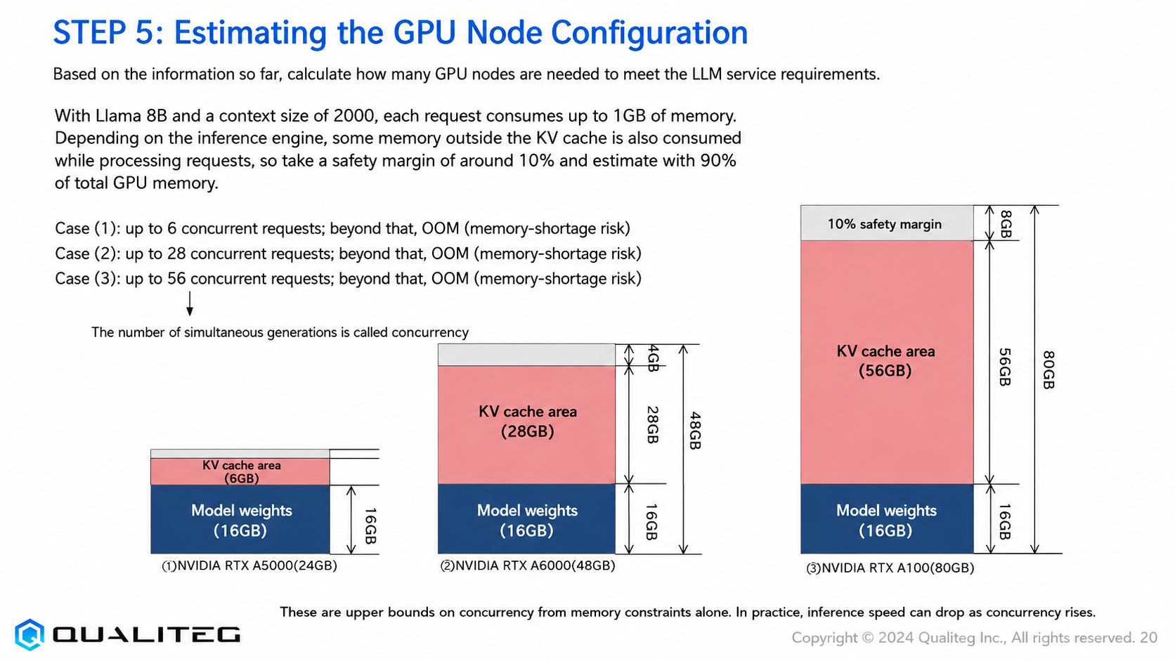
When building an LLM service, deciding which GPUs to use and how many is a critical decision. Using the Llama 8B model as an example, let's look at the relationship between GPU memory capacity and concurrent request capacity.
Understanding How GPU Memory Is Used
As a quick review:
in LLM inference, GPU memory is consumed for two main purposes
- Model weights: the memory that stores the LLM model itself
- KV cache: temporary memory that holds the conversational context with each user
Running Llama 8B at 16-bit precision, the model weights occupy about 16 GB of memory. This is a fixed memory cost: once loaded onto the GPU, it does not change.
The KV cache, on the other hand, is memory consumed per user request. With a context size of 2,000 tokens, each request consumes roughly 1 GB. In other words, how many user requests can be handled concurrently is determined by the size of the "KV-cache region" left over after loading the model weights.
With that in mind, let's look at the relationship between GPU memory capacity and concurrent requests.
Since GPU memory capacity is fixed by the GPU model, "which GPU to use" can be read as "how much GPU memory is available." (There are of course feature differences beyond memory capacity, but we will keep things simple here.)
GPU Memory Capacity vs. Number of Concurrent Requests
An 8B model is rarely used in production services these days, but suppose your requirements can be met with an 8B model. Let's compare running it on the following three NVIDIA GPUs.
RTX A5000 (24 GB) — Entry Model
After loading the 16 GB of model weights, roughly 6 GB remains (allowing a 10% safety margin). That corresponds to 6 concurrent requests — suitable for small deployments or single-department use.
RTX A6000 (48 GB) — Midrange Model
With the same model, 28 GB can be reserved for the KV cache, handling 28 concurrent requests. Ideal for midsize companies or shared use across multiple departments.
NVIDIA A100 (80 GB) — High-End Model
With a full 56 GB available for the KV cache, it can theoretically handle as many as 56 concurrent requests. Well suited to large internal services or systems with many users.
The A series belongs to the Ampere generation — somewhat dated as of 2025 — but (in hindsight) it was priced quite reasonably for its performance and is still in active service.
Mind the Gap Between Theoretical and Actual Performance
Remember that concurrency figures based on memory calculations are theoretical upper bounds. In practice, inference speed (token generation rate) gradually degrades as the number of concurrent requests grows, because the GPU's compute resources are shared across requests.
For example, if an A100 handles 50 concurrent requests, memory may be fine, yet the inference speed of each request may fall below target. The actual number of concurrent requests that can sustain the inference speed set in STEP 1 (e.g., 25 tokens/second) must be verified through load testing.
Selection Criteria
To summarize the key points when choosing a GPU:
- Know your peak concurrent request count
Can it cover the peak request volume calculated in STEP 2? - Factor in your inference-speed requirements
Inference speed drops as concurrency increases - Weigh cost performance
One expensive GPU, or several inexpensive ones? - Plan for scalability
Can it accommodate future user growth?
A Realistic Approach
If you are balancing budget and performance, a GPU in the RTX A6000 class is a realistic choice for many companies. It can handle a moderate number of concurrent requests (around 20-30) at a cost far below an A100.
For small deployments with few users, the RTX A5000 is also worth considering. Conversely, for large company-wide services or workloads that demand especially high inference speed, an A100 will justify the investment.
Whichever GPU you choose, do not stop at memory math: run real load tests and verify the inference speed and response times that directly shape the user experience.
Shrink the Model, or Add More GPUs?
In the previous section, we looked at the memory and concurrency of a single GPU.
We explained that when one GPU serves many requests, the inference speed per request drops. We have also seen that the model size a single GPU can host is constrained by its onboard GPU memory.
From here, let's look at techniques for using memory more efficiently and pushing inference speed further.
Real services need to run larger LLM models and handle many concurrent requests.
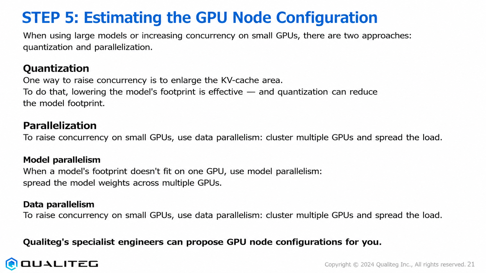
To design an efficient GPU node configuration in such cases, there are two main strategies: the quantization approach and the parallelization approach.
Let's look at the characteristics of each and where they apply.
Memory Efficiency Through Quantization
Quantization is a technique that dramatically reduces memory usage in exchange for a slight sacrifice in model precision. To increase concurrency you need to enlarge the KV-cache region, and reducing the model's footprint (the memory it occupies when loaded onto the GPU) is an effective way to do that.
For example, quantizing a standard 16-bit (FP16) model to 8-bit (INT8) or 4-bit (INT4) cuts the model footprint to one-half or one-quarter. That leaves room for more KV cache in the same GPU memory, allowing more requests to be processed concurrently.
Quantization is especially effective when:
- You want to raise concurrent request capacity within a single GPU
- Cost efficiency is a priority
- Throughput matters more than raw inference speed
That said, the lower the quantization level, the more generation quality may be affected, so it is important to find the right balance for your service requirements.
Although we speak of quantization as if it were one thing, there is no single method — several effective techniques have been proposed, and depending on the model architecture, some quantization methods can be used while others cannot. These days, when an open model is released, quantized versions tend to appear on Hugging Face within hours, so you can readily try community-quantized models without doing the work yourself.
Comparison of Major Quantization Algorithms
| Algorithm | Characteristics | Main advantages | Best suited for |
|---|---|---|---|
| AWQ | Weight quantization informed by activation characteristics | - High accuracy retention<br>- Per-channel mixed precision<br>- Large inference speedups | - Running large models within limited GPU memory<br>- Fast inference on NVIDIA GPUs |
| GPTQ | Layer-by-layer sequential quantization with error correction | - Relatively easy to implement<br>- Broad model compatibility<br>- Hugging Face support | - Inference with small batch sizes<br>- Applicable to a wide range of model types |
| bitsandbytes | Dynamic 8-bit/4-bit quantization | - Tight integration with PyTorch<br>- LLM.int optimizer<br>- Supports quantization during training | - Training and inference with Hugging Face models<br>- Fine-tuning large models on limited GPUs |
| GGUF | Unified model format and quantization | - Works well with CPU inference<br>- Open-source ecosystem<br>- Supports KV-cache quantization | - Inference on consumer hardware<br>- Llama/Mistral model families |
| QLoRA | Low-rank adaptation fine-tuning of quantized models | - Memory-efficient fine-tuning<br>- Direct tuning of quantized models<br>- Reduced memory requirements for large models | - Fine-tuning with limited GPU resources<br>- Combining quantization with fine-tuning |
Quantization Bit Widths and Their Effects
| Bit width | Memory reduction | Speedup | Accuracy impact | Recommended use |
|---|---|---|---|---|
| 8-bit | ~50% | 1.5-2x | Minimal | Production environments where high accuracy is essential |
| 4-bit | ~75% | 3-4x | Small to moderate | General LLM applications |
| 1+ bit | ~87-90% | 5-7x | Large | Extremely resource-constrained environments; when speed matters more than accuracy |
Choosing a Quantization Scheme
Choose the best algorithm and bit width based on your hardware, model type, required accuracy, and resource constraints. In today's LLM inference environments, 4-bit quantization offers the best balance of accuracy and efficiency. As 4-bit quantization has spread, NVIDIA GPUs have also begun to support GPU-native 4-bit quantization, contributing to even greater speedups.
Scaling Capacity Through Parallelization
The other important approach is parallelization: using multiple GPUs as a cluster to distribute the load. There are two main forms of parallelization
Model parallelism
This applies when the model's footprint is too large to fit on a single GPU. It is a technique for distributing the model weights across multiple GPUs. For example, a 70B-class model (70 billion parameters) cannot be loaded onto a single midrange GPU, so it is typically spread across several GPUs.
Model parallelism is effective when:
- Using large models (70B-100B and beyond)
- You want to operate a large model while preserving high generation quality
- You want to avoid the quality loss that quantization can introduce
Data parallelism
This applies when you want to increase concurrency with smaller GPUs. Multiple GPUs are clustered to distribute the load: each GPU is loaded with a copy of the same model, and different requests are dispatched to different GPUs.
Data parallelism is effective when:
- You need high throughput with small-to-midsize models (7B-13B class)
- You need to support many concurrent users
- You want to use resources efficiently
By combining these strategies appropriately, you can achieve a GPU node configuration that balances cost efficiency and performance. For concrete GPU node sizing, careful design by specialized engineers is recommended.
Our YouTube channel walks through concrete examples of parallelization — please have a look as well.
STEP 6: Load Testing
Once the GPU node configuration is decided, the next step is load testing: reproducing actual peak load to verify that the system meets its requirements. This is a critical step before deploying an LLM service to production.
Load Testing Overview
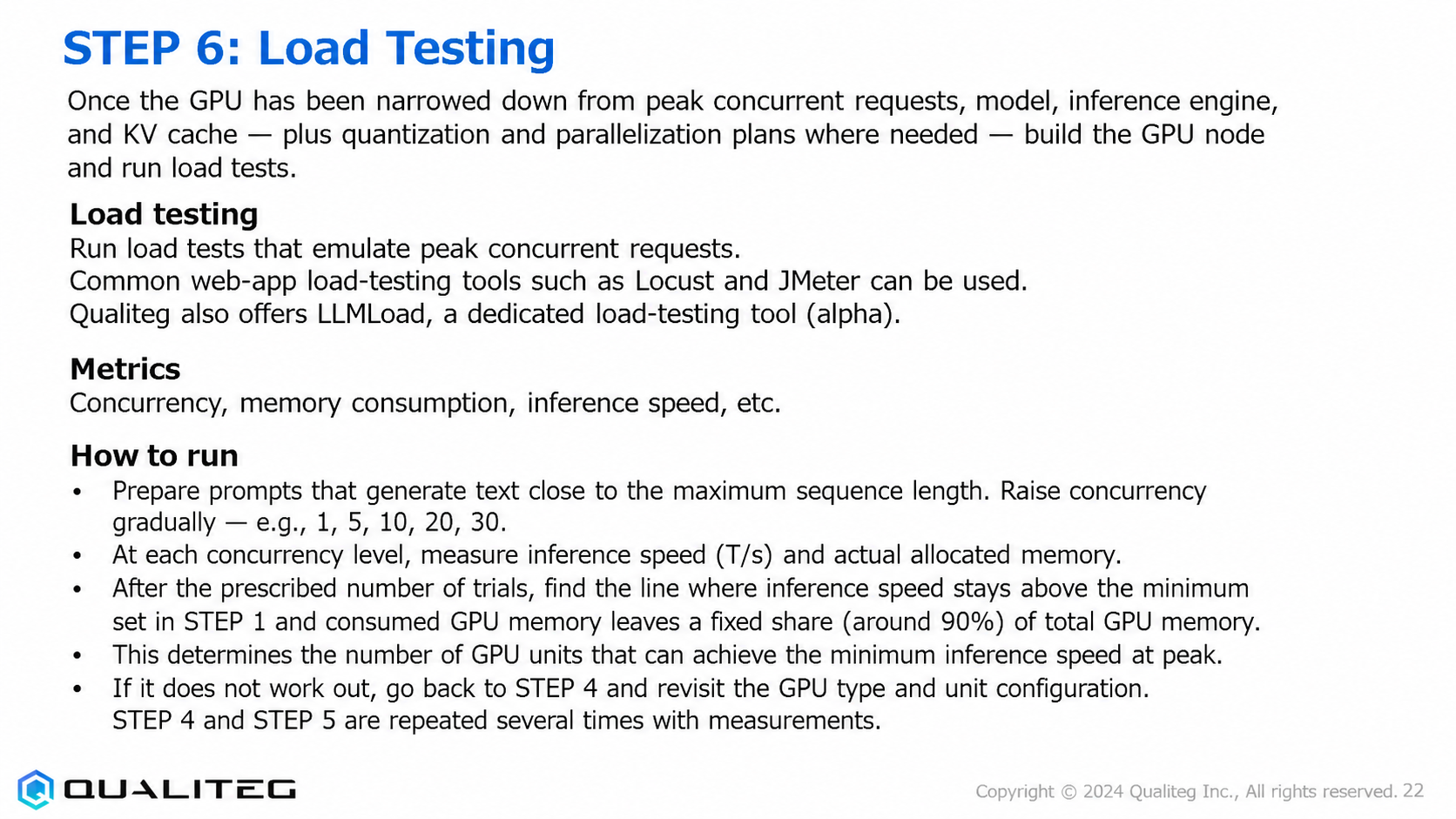
Using a load-testing tool that can emulate peak concurrent requests, verify performance from perspectives such as:
- Concurrent request capacity (concurrency)
- GPU memory consumption
- Inference speed (tokens/second)
- Response time
- System stability
General-purpose web-application load-testing tools such as Locust and JMeter can be used. Qualiteg also offers LLMLoad, a load-testing tool built specifically for LLMs (currently in alpha).
Test Plan and Measurement Procedure
For an effective load test, proceed as follows
- Prepare test prompts
Prepare prompts that drive text generation close to the maximum sequence length. Using prompts close to your real use cases is important. - Ramp up the load in stages
Gradually raise the number of concurrent requests — for example 1, 5, 10, 20, 30 — and measure performance at each step. - Measure at each stage
At each concurrency level, measure inference speed (tokens/second) and actual memory consumption. What matters most is staying above the minimum inference speed set in STEP 1 (e.g., 25 tokens/second) and keeping GPU memory usage within about 90% of total capacity. - Identify the limits
Through these measurements, determine the number of GPU units needed to achieve the minimum inference speed at peak load. - Identify and resolve problems
If the results fall short of expectations, go back to STEP 4 (inference engine selection) and STEP 5 (GPU node sizing) and revisit the GPU type and configuration. Repeat the tests as many times as necessary.
Load testing is not a mere formality; it is a process that directly determines the quality of the service. In particular, it yields valuable information for preventing trouble in production, such as pinpointing the maximum number of concurrent users and observing behavior when errors occur.
STEP 7: Trade-off Analysis
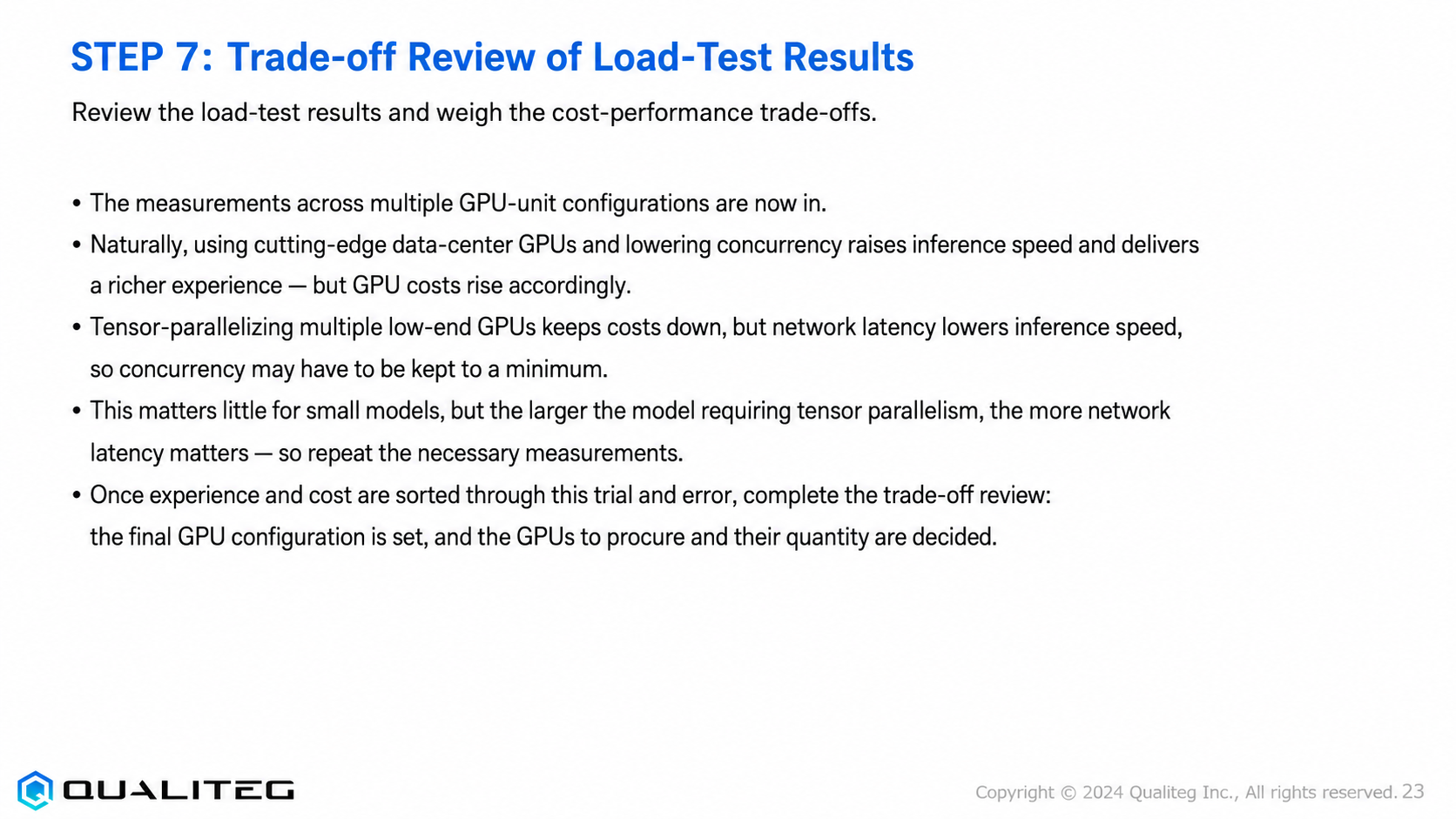
As the final step, weigh the cost-performance trade-offs based on the load-test results. This process is the key decision point for finalizing the GPU configuration.
Key Points of the Trade-off Analysis
Once measurements are in for several candidate GPU node configurations, evaluate them from perspectives such as the following
- High-end vs. lower-end GPUs
Naturally, using cutting-edge data-center GPUs (A100, H100, B200, and so on) allows high concurrency and a rich user experience, but GPU costs rise in proportion. Conversely, tensor-parallelizing several lower-end GPUs keeps costs down, but network latency may reduce inference speed — in which case you may need to keep concurrency to a minimum. - Considerations by model size
For small models (7B and below), tensor parallelism is rarely necessary; for large models (70B and above), the impact of network latency becomes a concern, so repeated, thorough measurement is required. - Balancing cost and experience
Ultimately, you will choose the configuration that delivers the best user experience within an acceptable cost envelope. It is important to consider both the initial cost (CAPEX) and the operating cost (OPEX).
Through this analysis, the final GPU configuration is decided and the number of GPUs to procure is fixed. The important thing is not to chase "maximum performance" or "minimum cost" in isolation, but to find the balance best suited to your service requirements.
Wrap-up: A Systematic Approach to LLM Inference Infrastructure Provisioning
Across this course, we have covered the seven steps for building an LLM inference infrastructure
- Define the inference speed
Set inference-speed targets based on service requirements - Estimate request volume
Calculate concurrent requests from user counts and usage patterns - Estimate the model's inference-time memory consumption
Calculate the model footprint and KV cache - Select an inference engine
Choose the engine best suited to the use case - Size the GPU node configuration
Consider quantization and parallelization strategies and design the configuration - Load testing
Verify performance under conditions close to real usage - Trade-off analysis
Make the final decision balancing cost and performance
Carrying out these steps systematically lets you build an LLM inference infrastructure with performance that is sufficient for your needs — without overinvesting.
Accurate estimation and planning in the early stages, in particular, are the key to avoiding major design changes and budget overruns later.
LLM technology evolves by the day, and inference technology is advancing rapidly. It is important to keep up with the latest developments while designing and building the inference infrastructure best suited to your needs. Continuous monitoring and optimization remain necessary once you enter the operational phase.
We hope this course serves as a useful guide for companies considering in-house LLM adoption. Please put this seven-step approach to work in planning cost-efficient LLM services that make the most of your GPU resources.
Qualiteg: Your Partner for LLM and AI Security
At Qualiteg, our engineering team has hands-on experience designing LLM inference and serving infrastructure. We do not treat inference engines as black boxes: our support for local LLM technology is grounded in deep knowledge of attention computation, KV-cache behavior, and more. From core technology to AI market analysis — "What configuration fits in our VRAM?", "vLLM or Hugging Face — what are the decision criteria?", "What is the fastest path to adapting an existing model to our domain?", "When to use open LLMs versus commercial LLMs?", "How do we build a secure local LLM configuration?", "How do we choose local LLMs and GPUs?", "GPU data-center demand and market forecasts", "AI market forecasts" — please feel free to reach out.